Summary:
We have investigated the relevant trend of the bolometric
correction (BC) at the cool-temperature regime of red giant stars and its
possible dependence on stellar metallicity. Our analysis relies on a wide
sample of optical-infrared spectroscopic observations, along the
3500 Å--2.5 μm wavelength range, for a grid of 92 red giant
stars in five (3 globular + 2 open) Galactic clusters, along the full
metallicity range covered by the bulk of the stars, -2.2 ≤ [Fe/H] ≤ +0.4.
Synthetic BVRcIcJHK photometry from the derived spectral energy
distributions allowed us to obtain robust temperature (Teff) estimates
for each star, within ± 100 K or less. According to the appropriate temperature
estimate, black-body extrapolation of the observed spectral energy distribution (SED)
allowed us to assess the unsampled flux beyond the wavelength limits of our survey.
For the bulk of our red giants, this fraction amounted to 15% of the total bolometric
luminosity, a figure that raises up to 30% for the coolest targets
(Teff ≤ 3500 K). Allover, we trust to infer stellar Mbol
values with an internal accuracy of a few percent. Even neglecting any correction
for lost luminosity etc. we would be overestimating Mbol by ≤ 0.3 mag,
in the worst cases. Making use of our new database, we provide a set of fitting functions for
the V and K BC vs. Teff and vs. (B-V) and (V-K) broad-band colors,
valid over the interval 3300 K ≤ Teff ≤ 5000 K,
especially suited for Red Giants.
The analysis of the BCV and BCK estimates along the wide range of
metallicity spanned by our stellar sample show no evident drift with [Fe/H].
Things may be different for the B-band correction, where the blanketing effects
are more and more severe. A drift of Δ (B-V) vs. [Fe/H] is in fact
clearly evident from our data, with metal-poor stars displaying a "bluer"
(B-V) with respect to the metal-rich sample, for fixed Teff.
Our empirical bolometric corrections are in good overall agreement with most of
the existing theoretical and observational determinations, supporting the
conclusion that (a) BCK from the most recent studies are reliable within
≤ ±0.1 over the whole color/temperature range considered in this paper, and
(b) the same conclusion apply to BCV only for stars warmer than ~3800 K.
At cooler temperatures the agreement is less general, and MARCS models
are the only ones providing a satisfactory match to observations, in particular
in the BCV vs. (B-V) plane.
|
| Table 1 - Cluster properties and stellar database for cluster M 15 | (ASCII) |
|
| Table 2 - Cluster properties and stellar database for cluster M 2 | (ASCII) |
|
| Table 3 - Cluster properties and stellar database for cluster M 71 | (ASCII) |
|
| Table 4 - Cluster properties and stellar database for cluster NGC 188 | (ASCII) |
|
| Table 5 - Cluster properties and stellar database for cluster NGC 6791 | (ASCII) |
|
| Table 6 - Logbook of TNG observations along 2003 | (ASCII) |
|
| Table 7 - Magnitude residuals between observed and theoretical magnitudes | (ASCII) |
|
| Table 8 - Standard synthetic photometry from SED of target stars in globular clusters M 71, M 15, and M 2 | (ASCII) |
|
| Table 9 - Standard synthetic photometry from SED of target stars in open clusters NGC 188 and NGC 6791 | (ASCII) |
|
| Table 10 - Stellar outliers of our sample in the different photometric bands | (ASCII) |
|
| Table 11 - Inferred temperatures, bolometric magnitude and bolometric corrections for target stars in globular clusters M 71, M 15, and M 2 | (ASCII) |
|
| Table 12 - Inferred temperatures, bolometric magnitude and bolometric corrections for target stars in open clusters NGC 188 and NGC 6791 | (ASCII) |
|
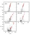 |
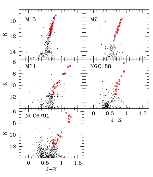
Figure 1 -
Apparent c-m diagram of the five clusters included in our analysis,
according to 2MASS J and K photometry. Big squares along the red giant branch
mark the selected targets in our sample.
|
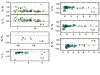 |
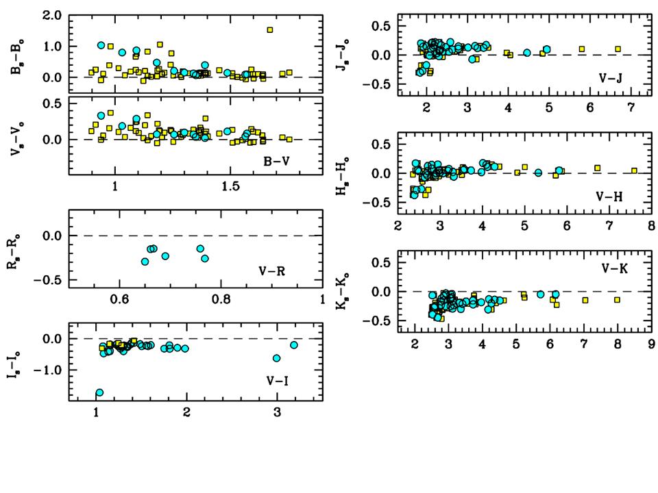
Figure 2 -
The B,V,Rc,Ic,J,H,K magnitude residuals between synthetic
and observed magnitudes (in the sense "syn"−"obs") for the 94 stars
in our sample.plotted vs. literature colors, according to the data of
Table 2 to 6.
Synthetic magnitudes derived from the numerical integration of the observed
SED with the Johnson-Cousins filters. All the available photometry has been accounted
for. Some stars with multiple V datasets appear therefore twice in the
plots and are singled out by dot and square markers, respectively.
|
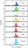 |
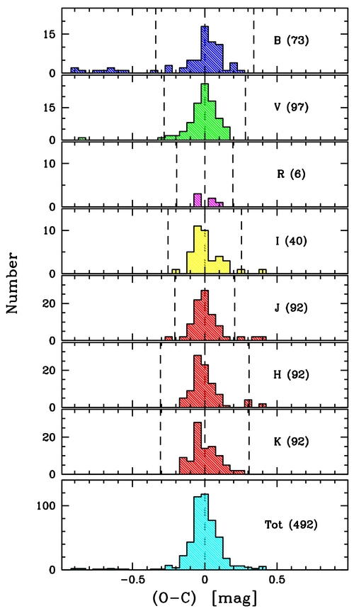
Figure 3 -
The histogram of magnitude residuals for the data of Fig. 1,
after correction for the systematic offsets, according to Table 7.
A total of 492 measures
have been accounted for, as labelled in the global histogram of the bottom panel,
including multiple photometry sources in the literature from Tables 2 to 6.
Dashed vertical lines mark the ± 3σ clipping edges, according to our
iterative procedure, as devised in Sec. 3.2. Mag residuals are in the sense
"obs"−"syn". After outliers rejections, the global sample of 458 measurements
has, on average, σ(Δmag) = ± 0.095 (see Table 7).
|
 |
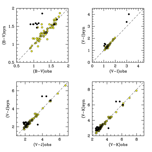
Figure 4 -
Color distribution of photometric outliers, according to our 3σ clipping
procedure (see Fig. 3). Target location for the whole star sample in the synthetic
vs. observed color planes are displayed, with dark solid dots marking the "dropped"
objects (see Table 10).
|
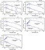 |
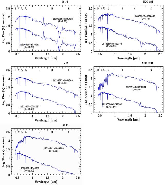
Figure 5 -
The resulting (dereddened) SED according to optical and infrared observations
for an illustrative stellar subset of each cluster, including the brightest (and
roughly coolest) and faintest (i.e. warmest) stars. Note, especially for the
M 15 stars, the strong impact of telluric water vapor bands at 1.38 and 1.88 μm.
Their variability along the observing nights prevented, in some cases, any accurate
cleaning procedure. See discussion in Sec. 3.1.
|
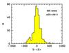 |
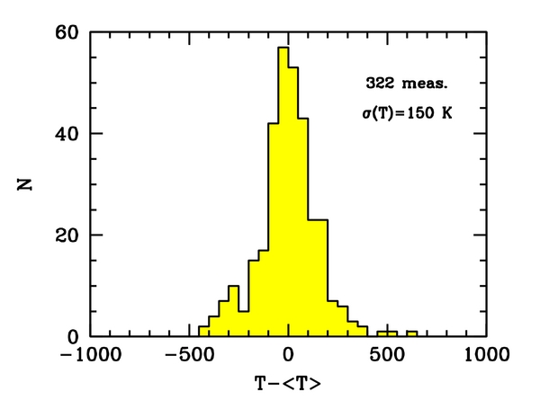
Figure 6 -
Histogram of temperature difference for all the data reported
in Tables 8 and 9 (cols. 6 to 9) with respect to the adopted
mean estimate (<T> of col. 10). A total of 322 entries
are available for the whole stellar sample. The resulting distribution gives
a direct measure of the internal uncertainty of our temperature scale,
amounting to σ(Teff) = ±150 K for the standard individual
estimate.
|
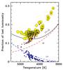 |
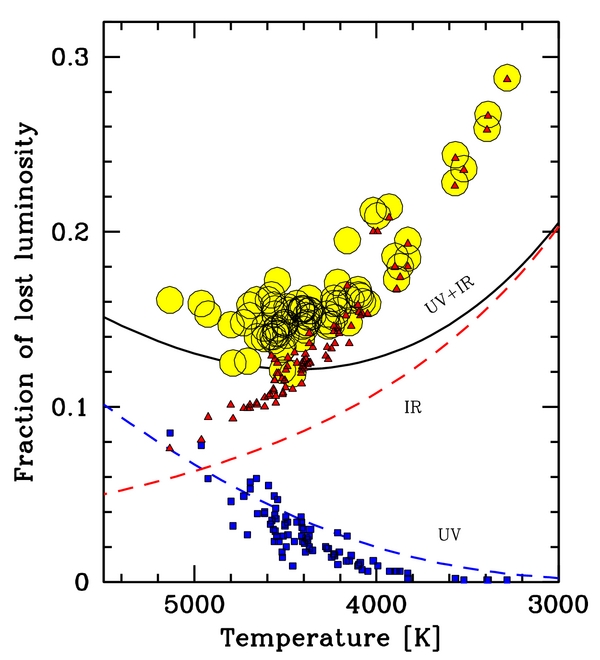
Figure 7 -
Estimated fraction of unsampled stellar luminosity for the
stars in our sample (big solid dots). The relative contribution to
stellar bolometric luminosity from lost emission at short (i.e. for
λ ≤ 4000Å, small square markers on the plot) and long (i.e. for
λ ≥ 2.25μm, small triangles) wavelength is sized up by extrapolating
the observed SED with two black-body (BB) "wings" at fixed <T>,
as from col. 10 of Table 11 and 12.
The same excercise is carried out for a full BB spectrum along the
5500-3000 K temperature range (dashed lines labelled "UV" and "IR" for
the short and long wavelength contribution, respectively, together with their
summed contribution, as in the solid line). Compared to a plain BB case, note
that real stars at cool temperatures display a brighter IR luminosity.
|
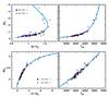 |
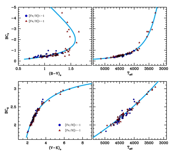
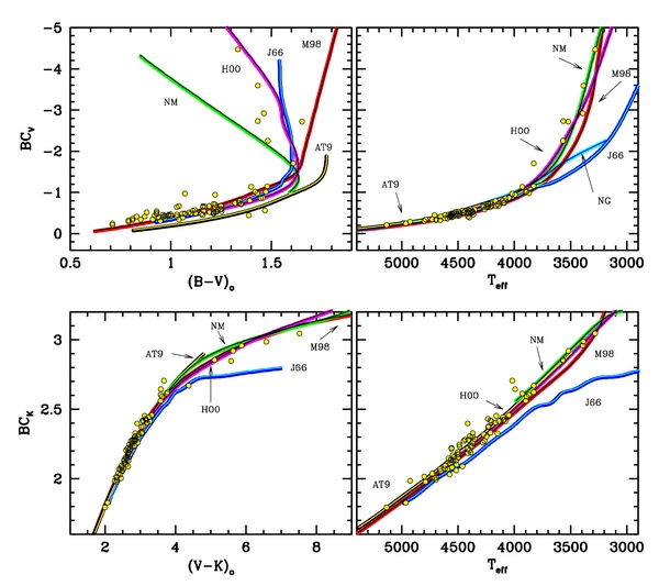
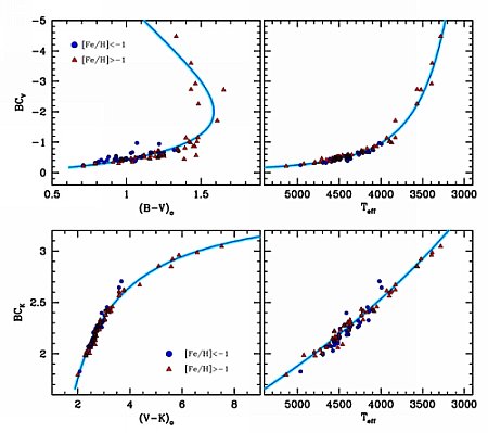
Figure 8 -
The BC vs. color (left panels) and BC vs. Teff (right
panels) distribution of our stellar sample (dots and triangles, for
metal-poor and metal-rich stars, respectively). Synthetic
colors have been corrected for Galactic reddening.
Solid lines are our derived calibrations, according to the set of
eqs. (4) and (5).
|
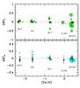 |
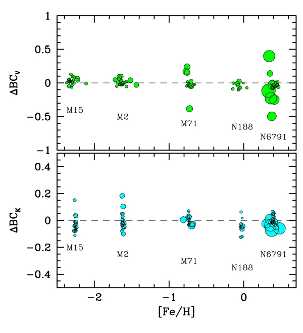
Figure 9 -
The distribution of BC residuals for our stellar sample vs.
cluster metallicity. The displayed ΔBC is intended
as the difference between the values of cols. 12 and 13 of Tables 11
and 12 and the output of eq. (4) entering with the adopted
effective temperature of stars, as in col. 10 of the tables. Note the lack of
any evident correlation with [Fe/H], as discussed in more detail in Sec. 5.2.
Data in the plot have been slightly spread around the cluster [Fe/H] value
for better reading. Dot size is inversely proportional to star temperature
(i.e. bigger dots = cooler red giants).
|
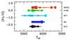 |
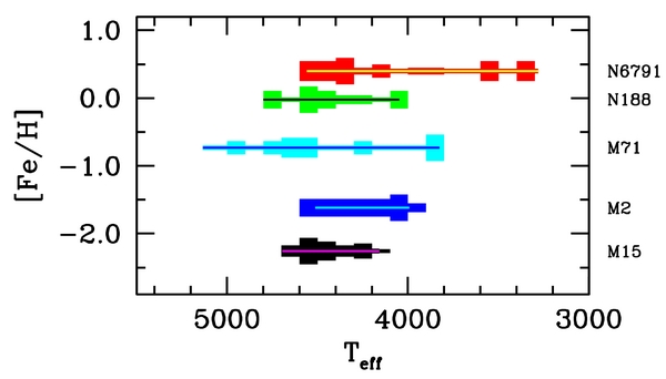
Figure 10 -
Temperature distribution of red-giant stars in each of the five clusters
of our sample, according to Table 11 and 12. Line tickness
is proportional to the star density along the spanned temperature range.
Note that only cluster NGC 6791 contains stars cooler than ~3800 K.
|
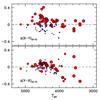 |
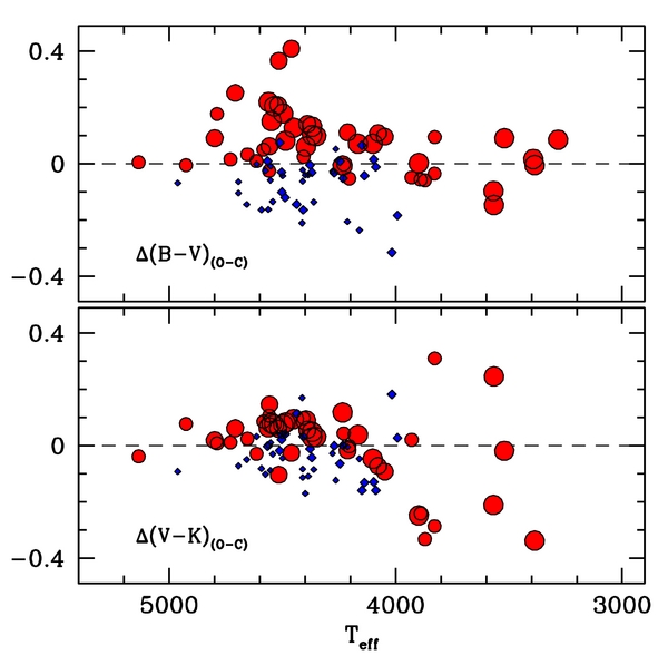
Figure 11 -
Residual (B-V) and (V-K) distribution vs. stellar temperature for stars
in Table 11 and 12. Color residual is computed as a difference between
observed and expected values by entering eq. (5) with the BC output
of eq. (4). Metal-poor and metal-rich stars are singled out by diamonds
and dot markers, respectively, taking the value [Fe/H] = −1.0 dex
as a reference threshold. Marker size increases with [Fe/H], throughout.
|
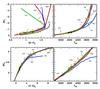 |
Figure 12 -
Same as Fig. 8, but comparing our data with different theoretical
and empirical calibrations from Johnson (1966) ("J66" labels), Bertone et al. (2004)
using Atlas9 (Kurucz 1992, "AT9") and NextGen (Hauschildt et al. 1999, "NG")
synthesis codes for model atmosphere computation, Montegriffo et al. (1998, "M98"),
and Houdashelt et al. (2000, "H00") using Marcs theoretical code by
Bell & Gustafsson (1978), and its updated version (NMarcs), as in
Plez et al. (1992) and Bessell et al. (1998, "NM").
|