Back to article listing

Back to article listing |
|
Shortcut to the SSP models |
| Buzzoni, A.: | |||
| "Energetic constraints to chemo-photometric evolution
of spiral galaxies", 2011, MNRAS, 415, 1155 | |||
|
|
Summary:
The problem of chemo-photometric evolution of late-type
galaxies is dealt with relying on prime physical arguments of energetic
self-consistency between chemical enhancement of galaxy mass, through
nuclear processing inside stars, and luminosity evolution of the system.
Our analysis makes use of the Buzzoni (2002, 2005)
template galaxy models along the Hubble morphological sequence.
The contribution of TypeII and Ia SNe is also accounted for in our
scenario.
Chemical enhancement is assessed in terms of the so-called
"yield metallicity" (Z), that is the metal abundance of processed
mass inside stars, as constrained by the galaxy photometric history.
For a Salpeter IMF, Z ∝ t0.23
being nearly insensitive to the galaxy star formation history.
The ISM metallicity can be set in terms of Z, and just modulated
by the gas fraction and the net fraction of returned stellar mass (f).
For the latter, a safe upper limit can be placed, such as f ≤ 0.3
at any age.
The comparison with the observed age-metallicity relation allows us to to set a firm
upper limit to the Galaxy birthrate, such as b ≤ 0.5, and to
the chemical enrichment ratio ΔY/ΔZ ≤ 5.
About four out of five stars in the solar vicinity are found
to match the expected Z figure within a factor of two, a feature
that leads us to conclude that star formation in the Galaxy must have
proceeded, all the time, in a highly contaminated environment where returned
stellar mass is in fact the prevailing component to gas density.
The possible implication of the Milky Way scenario for the more general picture of
late-type galaxy evolution is dicussed moving from three relevant
relationships, as suggested by the observations. Namely, i) the down-sizing
mechanism appears to govern star formation in the local Universe; ii)
the "delayed" star formation among low-mass galaxies, as implied by the inverse
b-Mgal dependence, naturally leads to a more copious gas fraction
when moving from giant to dwarf galaxies; iii) although lower-mass galaxies
tend more likely to take the look of later-type spirals, it is mass, not
morphology, that drives galaxy chemical properties.
Facing the relatively flat trend of Z vs. galaxy type, the increasingly
poorer gas metallicity, as traced by the [O/H] abundance of HII regions
along the Sa → Im Hubble sequence, seems to be mainly the result of the
softening process, that dilute enriched stellar mass within a larger fraction of
residual gas.
The problem of the residual lifetime for spiral galaxies as active
star-forming systems has been investigated. If returned mass is
left as the main (or unique) gas supplier to the ISM, as implied by the Roberts
timescale, then star formation might continue only
at a maximum birthrate bmax << f/(1-f) ≤ 0.45, for a Salpeter IMF.
As a result, only massive (Mgal ≥ 1011 Msun) Sa/Sb
spirals may have some chance to survive ~30% or more beyond a Hubble time.
Things may be worse, on the contrary, for dwarf systems, that seem currently on
the verge of ceasing their star formation activity unless to drastically
reduce their apparent birthrate below the bmax threshold.
|
| Pick up the paper at Astro-ph/1105.0428 | Local link to the PDF version (230 Kb) | ||
| Enhanced HTML/PDF version at the MNRAS site (*) | |||
| (*)May require access password |
| ||
| ||
| ||
| ||
| ||
|
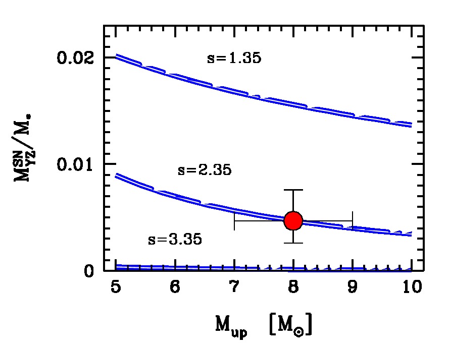 |
Figure 1 -
The expected fraction of enriched stellar mass provided by the
SNII events according to three different IMF power-law indices
(Salpeter case is for s = 2.35), and for a different value of
the SN triggering mass, Mup. The consensus case is marked by
the big dot on the Salpeter curve. Vertical error bars derive from
eq. (14).
|
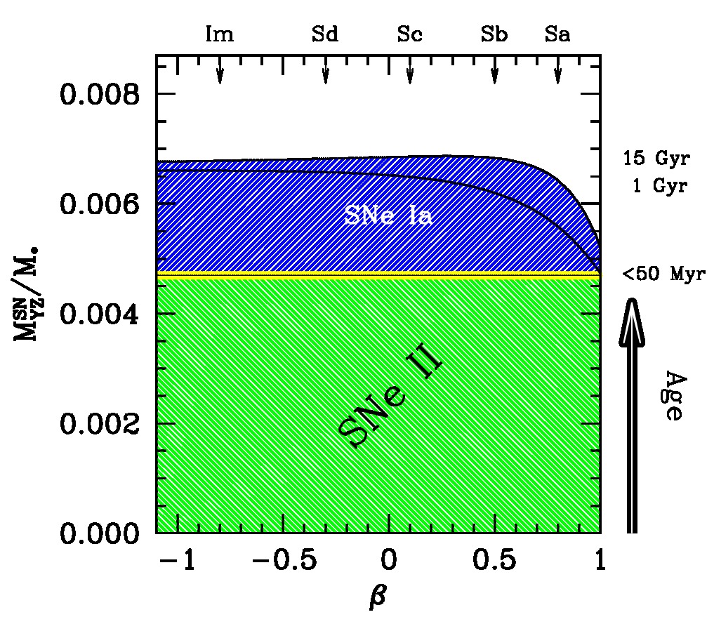 |
Figure 2 -
The chemical enrichment from SN contribution according
to the different components. Note the prevailing role of core-collapsed objects
(i.e. SNII) along the early stages of galaxy evolution (t ≤ 50 Myr,
see labels to the right axis). The total SNIa component adds then a further 0.2 dex
to galaxy metallicity, mostly within the first Gyr of life.
|
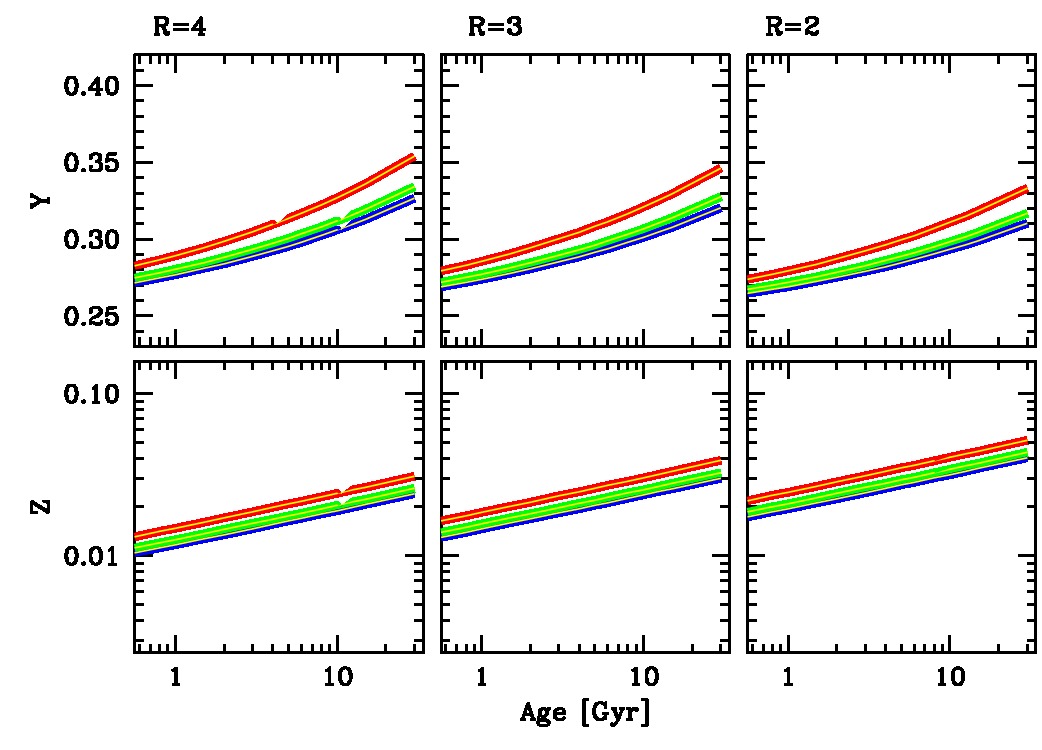 |
Figure 3 -
Yield chemical abundance for the CSP set of Table 3. Theoretical
output is from eq. (24), assuming a range
for the enrichment ratio R = ΔY/ΔZ = 3 ±1, according to the
label in each panel. Note the nearly insensitive response of
both Y and Z to the SFR details.
|
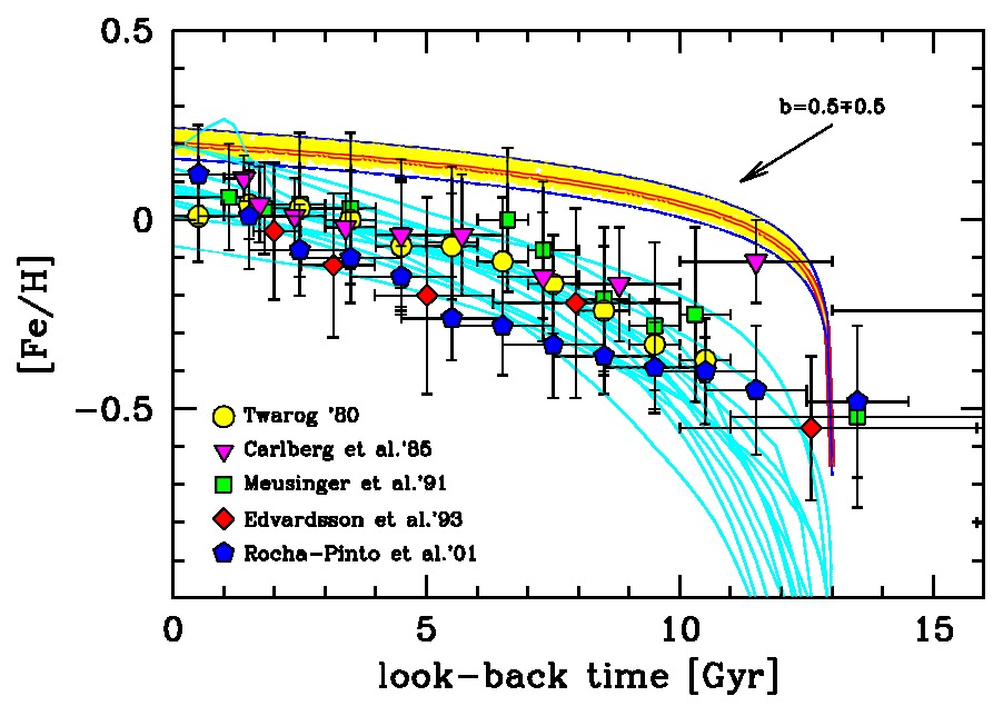 |
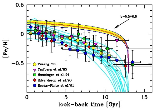
Figure 4 -
The solar-neighbourhood AMR, according to different
observing surveys, as labelled in the plot. In particular, the works of
Twarog (1980) (dots), Carlberg et al. (1985) (triangles), Meusinger,
Stecklum & Reimann (1991) (squares), Edvardsson et al. (1993) (diamonds),
and Rocha-Pinto et al. (2000) (pentagons) have been considered. Observations are
compared with model predictions from several theoretical codes (the shelf of thin curves;
see Fig. 5 for a detailed source list).
The expected evolution of yield metallicity, according to eq. (27),
is also displayed, assuming [Fe/H] = log(Z/Zsun), and
a birthrate b = 0.5±0.5, as labelled on the curve. A current
age of 13 Gyr is adopted for the Milky Way. See text for a full discussion.
|
 |
Figure 5 -
Representative parameters for the observed (dots) and predicted (squares)
AMR for the solar neighborhood. The theoretical works by
Matteucci & Fracois (1989) (labelled as "MF" on the plot), Wyse & Silk (1989)
(WS1 and WS2, respectively for a Schmidt law with n = 1 and 2),
Carigi (1994} (C), Pardi & Ferrini (1994) (PF), Prantzos & Aubert (1995)
(PA), Timmes, Woosley & Weaver (1995) (TWW), Giovagnoli & Tosi (1995)
(GT), Pilyugin & Edmunds (1996) (PE), Mihara & Takahara (1996)
(MT), Chiappini, Matteucci & Gratton (1997) (CMG), Portinari, Chiosi & Bressan
(1998} (PCB), Boissier & Prantzos (1999) (BP), and Alibes, Labay & Canal (2001)
(ALC) have been acounted for, including the expected output from the Z law
of eq. (27) (square marker labelled as "B"). The Milky Way is assumed to
be 13 Gyr old for every model. The theoretical data set is also compared with
the observations, according to the surveys of Twarog (1980) (dot number "1"),
Carlberg et al. (1985) ("2"), Meusinger et al. (1991) ("3"), Edvardsson et al. (1993)
("4"), Rocha-Pinto et al. (2000) ("5"), and Holmberg et al. (2007) ("6").
An AMR in the form [Fe/H] = ζ log t9 + ω,
is assumed, throughout.
The displayed quantities are therefore the slope coefficient ζ, vs. the
expected metallicity at t = 10 Gyr, namely [Fe/H]10 = ζ+ω.
Note that models tend, on average, to predict a sharper chemical evolution
with respect to the observations. This leads, in most cases, to a steeper slope
ζ and a slightly higher value for [Fe/H]10. See the text for a
discussion of the implied evolutionary scenario.
|
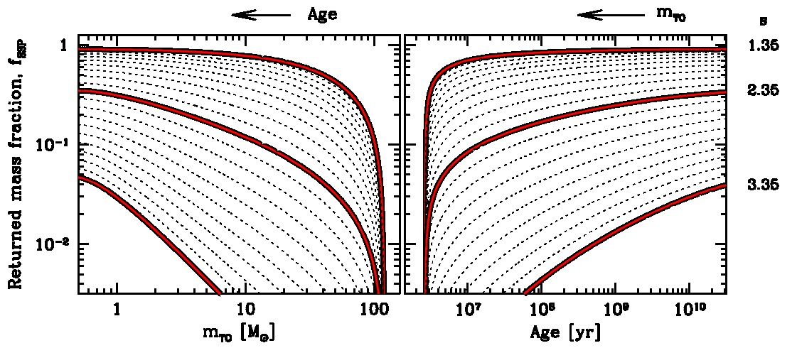 |
Figure 6 -
The expected fraction FSSP = Mret/Mtot
of stellar mass returned to the ISM for a set of SSPs, with changing the IMF power-law
index (s), as labelled to the right. The evolution is traced both vs. SSP
age and the main-sequence Turn Off stellar mass (mTO), the latter via
eq. (3) of Buzzoni (2002).
The relevant case for a Salpeter IMF (s = 2.35) and two indicative variants
for giant- (s = 1.35) and dwarf-dominated (s = 3.35) SSPs are
singled out in both panels, while the thin dotted curves account for the intermediate
cases, by steps of Δs = 0.05 in the IMF index.
|
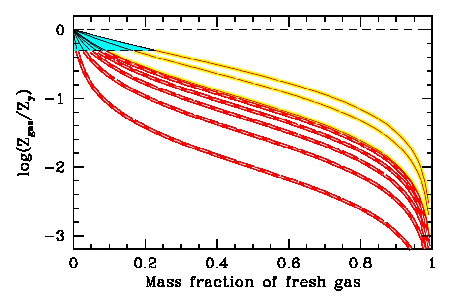 |
Figure 7 -
The output of eq. (29) is displayed vs. the mass
fraction of fresh primordial gas (G). The two shelves of curves
assume the fraction f of returned stellar mass as a free parameter.
The lower shelf (dashed curves) is for f = 0.01 → 0.09
by steps of Δf = 0.02, while the upper shelf of curves (solid lines) cover the
f range from 0.1 to 0.3, by steps of Δf = 0.1.
The shaded area within −0.3 ≤ log (Zgas/Z≤ 0
single out the allowed f-G
combinations that may account for the observed metallicity spread of
stars in the solar neighborhood.
|
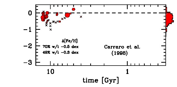 |
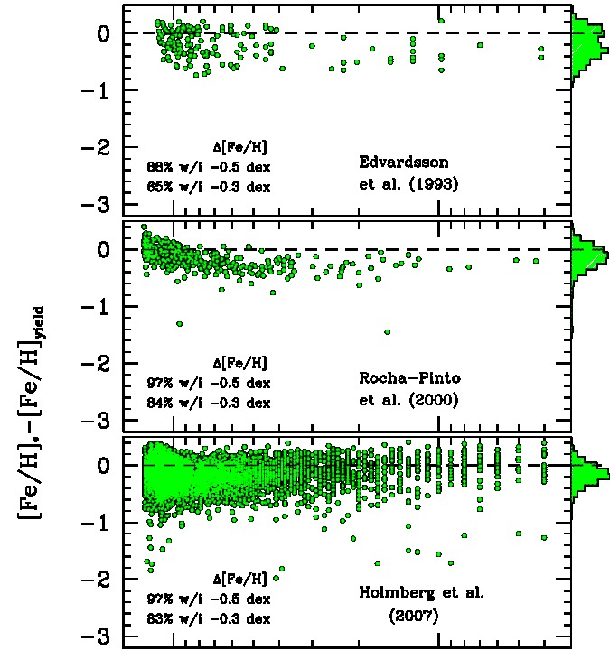
Figure 8 -
The observed metallicity distribution of stars
in the solar neighbourhood. The displayed quantity is
Δ[Fe/H] = [Fe/H]* − [Fe/H]yield
≡ log (Zgas/Z).
Different stellar samples have been
considered from the work of Edvardsson et al. (1993),
Rocha-Pinto et al. (2000), and Holmberg et al. (2007), from top to bottom,
as labelled in each panel. The lower panel displays the same trend
for a sample of open stellar clusters, after Carraro et al. (1998).
The different Galacticentric distance for these systems is indicatively
marked by the dot size (i.e. the smallest the dot, the largest the
distance from the Galaxy center). For each distribution,
the relative fraction of stars within a −0.3 and −0.5 dex
Δ[Fe/H] residual is reported in each panel. A cumulative histogram of the data
is also displayed, along the right axis, in arbitrary linear units.
|
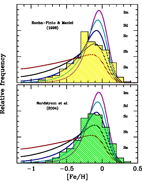 |
Figure 9 -
The [Fe/H] distribution of G-dwarf stellar samples in the solar
neighborhood (shaded histograms), according to Rocha-Pinto et al. (2000) (upper panel),
and Nordstrom (2004) (lower panel), is compared with the expected
yield-metallicity distribution accounting for the different star-formation
histories as for the disk stellar population of Buzzoni (2005) template
galaxies along the Hubble sequence (solid curves, as labelled on the plot).
A roughly constant stellar distribution in the Z domain leads to
an implied birthrate of the order of b~0.6, as pertinent to
Sbc galaxies (see Table 2 for a reference).
|
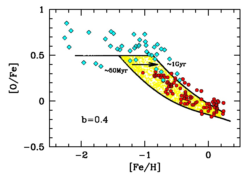 |
Figure 10 -
The [O/Fe] distribution of stars in the Milky Way is displayed acording to
the Jonsell et al. (2005) (diamonds) and Edvardsson et al. (1993) (dots) data samples,
respectively for the halo and disk stellar populations. Our model output, according
to eq. (46) is superposed (solid lines), for a representative birthrate
b = 0.4, and for a range of SNIa delay time Δ from ~50 Myr
to ~1 Gyr, as discussed in Sec. 2.2.
|
 |
Figure 11 -
The gas metallicity of 15 Gyr disk stellar populations according to
the Arimoto & Jablonka (1991) (AJ91) models (solid line with diamonds) is displayed
together with the expected predictions from eq. (31) (shaded area)
for a range of returned mass fraction f between 0.07 and 0.3, as labelled on
the plot. For tighter self-consistency in our
comparison, the adopted gas fraction Gtot for our model
sequence matches the corresponding figures of AJ91 models, while
yield metallicity derives from eq. (27) for the relevant
birthrate values of the Buzzoni (2005) template models
along the Sa → Im morphological sequence (solid line with dots).
|
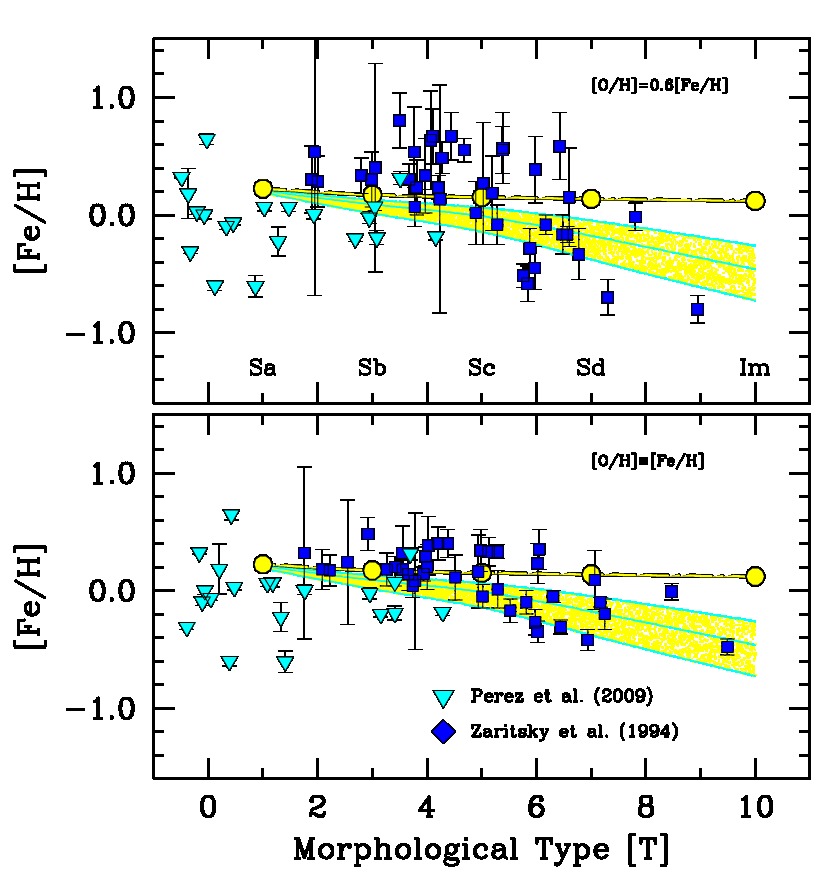 |
Figure 12 -
[Fe/H] metallicity for the two galaxy samples of Perez et al. (2009)
(triangles) and Zaritsky et al. (1994) (squares), compared with the yield and gas
metallicity figures (solid line with dots and shaded area) as from Fig. 11.
While the Perez et al. (2009) estimates derive from Lick indices tracing the
galaxy stellar population, in case of Zaritsky et al. (1994) the [Fe/H]
derives from the Oxygen abundance of galaxy HII regions, by adopting
log (O/H)sun = 8.83 for the Sun (Grevesse & Sauval 1998).
Two cases are envisaged, in this regard, assuming that Oxygen straightly
traces Iron (and the full metallicity), as in lower panel or, more
realistically, that a scale conversion does exist such as
[O/H] = 0.6 [Fe/H],
as suggested by the observation of disk stars in the Milky Way
(Clegg et al. 1981, Bessell et al. 1991, Edvardsson et al. 1993). A little
random scatter has been added to the morphological T class of the points
in each panel for better reading.
|
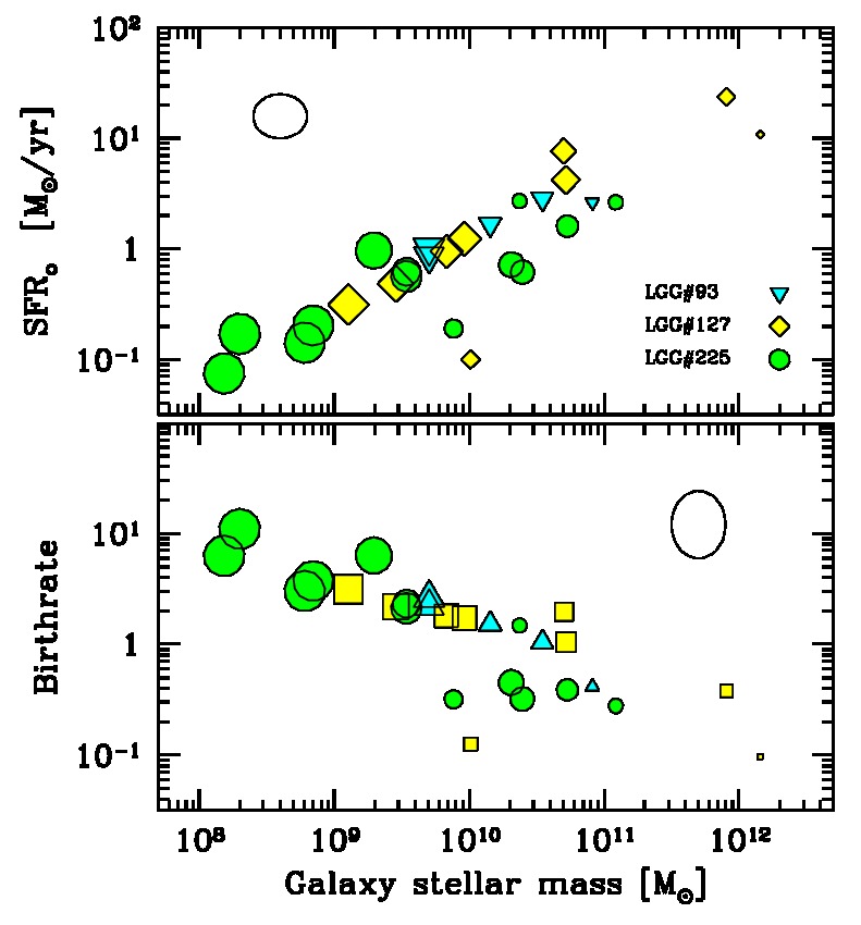 |
Figure 13 -
The inferred star-formation properties of the spiral-galaxy sample
by Marino et al. (2010), referring to three Local-Group Analogs from the LGG
catalog Garcia (1993), as marked and labelled on the plot.
Marker size indicates galaxy morphology along the RC3 T-class sequence
(the biggest markers are for Sd/Im galaxies with T~10, while the
smallest are for Sa systems with T~1). Current SFR derives
from GALEX NUV fluxes, dereddened as discussed in the text, and calibrated
according to Buzzoni (2002).
On the contrary, Galaxy stellar mass is computed from the relevant M/LB
ratio, as from the Buzzoni (2005) template galaxy models.
The birthrate assumes for all galaxies a current age of 13 Gyr.
The small ellipses in each panel report the typical uncertainty figures,
as discussed in the text. All the relevant data for this sample are summarized
in Table 5. Note the inverse relationship between b and
M*gal, as in the down-sizing scenario for galaxy formation.
|
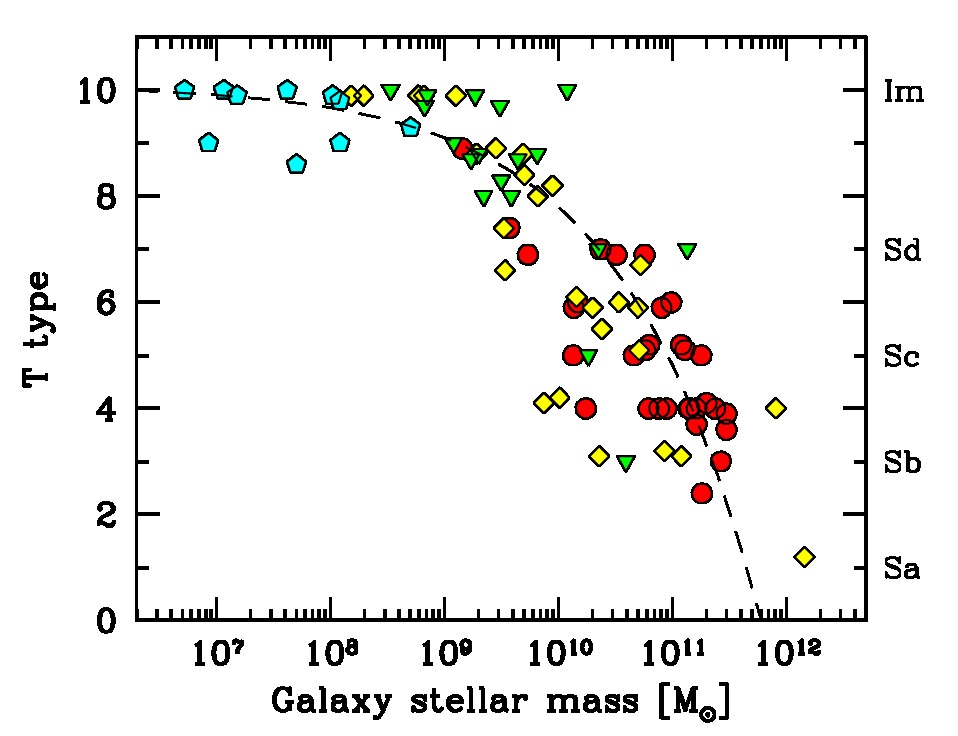 |
Figure 14 -
The observed relationship between morphological RC3 class T
and galaxy stellar mass according to four different galaxy samples
from the work of Garnett (2002) (dots), Marino et al. (2010)
(diamonds), Kuzio de Naray et al. (2004) (triangles) and Saviane et al. (2008) (pentagons)
(see Table 5 and 6 for details).
The value of M*gal derives from B photometry for
the Garnett (2002), Kuzio de Naray et al. (2004) and Marino et al. (2010) galaxies,
and from H absolute magnitudes for the Saviane et al. (2008) sample, throught the
appropriate M/L ratio, according to Buzzoni (2005).
Equation (49) provides a fair representation of the data, as
displayed by the dashed curve. As already pointed out also by Roberts & Haynes (1994)
one has to remark, however, the notable dispersion in mass among Sbc galaxies.
|
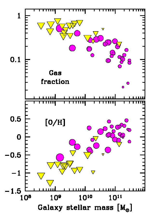 |
Figure 15 -
Mass fraction of gas and Oxygen abundance of HII regions for the
Garnett (2002) (dots) and Kuzio de Naray et al. (2004) (triangles) galaxy samples of
Table 6. Marker size is propotional to
the galaxy morphological class T (the biggest markers are for Sd/Im galaxies
with T~10, while the smallest are for Sa systems with T~1).
Gas fraction accounts for both atomic and molecular phase. Note the inverse relationships
of the data versus galaxy stellar mass, the latter as derived from the relevant
M/L ratio (see, again, Table 6 for details).
|
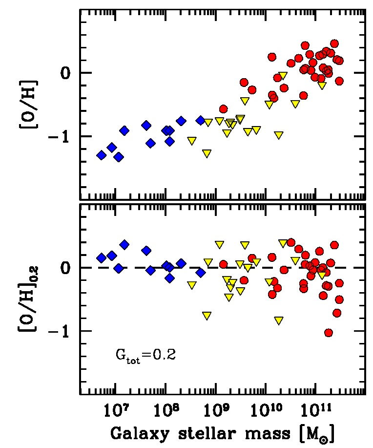 |
Figure 16 -
Upper panel: Oxygen abundance from HII regions for the galaxy
samples of Garnett (2002) (dots), Kuzio de Naray et al. (2004) (triangles) and
Saviane et al. (2008) (diamonds).
A nice correlation is in place with galaxy stellar mass, where low-mass systems
appear richer in gas (see Fig. 15) and poorer in metals.
Once accounting for the different gas fraction among the galaxies, and rescale
Oxygen abundance to the same gas fraction (Gtot = 0.2,
as in the indicative example displayed in the lower panel), note that most of the
[O/H] vs. M*gal trend is recovered, leaving a nearly
flat [O/H] distribution along the entire galaxy mass range, as predicted by
the nearly constant yield-metallicity of the systems.
|
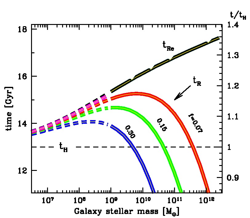 |
Figure 17 -
The lifetime of spiral galaxies as active star-forming systems,
better recognized as the Roberts & Haynes (1963) time, is computed along the full
mass range of the systems.
The definite consumption of the primordial gas reservoir, as in the
original definition of the timescale, tR, derives from eq. (54),
by parameterizing with the current fraction of returned stellar mass, f.
Present-day galaxies are assumed to be one Hubble time old
(tH ~13 Gyr, see
the left scale on the vertical axis). If returned stellar mass is also
included in the fuel budget, to further extend star formation, the the
"extended" Roberts time, tRe derives from eq. (55).
In both equations, the distinctive birthrate relies on the observed down-sizing
relationship of eq. (47), while the gas fraction available to
present-day galaxies is assumed to obey eq. (50), eventually
extrapolated for very-low mass systems (i.e.
M*gal ≤ 109Msun)
(dashed curves in the plot). Note, for the latter, that they seem on the verge
of definitely ceasing their star formation activity, while only
high-mass galaxies (M*gal ≥ 1011Msun) may still have chance
to extend their active life for a supplementary 30-40% lapse of tH.
See text for a full discussion.
|
Back to article listing |
|
Shortcut to the SSP models |
| AB/Oct 2011 |
|
|