Back to article listing

Back to article listing |
|
Shortcut to Space Stuff |
| Buzzoni, A., Altavilla, G., and Galleti, S.: |
| "Optical tracking of deep-space spacecraft in Halo L2 orbits and beyond:
the Gaia mission as a pilot case", 2016, Advances in Space Research, 57, 1515 |
|
|
Summary:
We tackle the problem of accurate optical tracking of distant man-made probes, on Halo orbit
around the Earth-Sun libration point L2 and beyond, along interplanetary transfers.
The improved performance of on-target tracking, especially when observing with small-class
telescopes is assessed providing a general estimate of the expected S/N ratio in spacecraft
detection.
The on-going Gaia mission is taken as a pilot case for our analysis, reporting on fresh
literature and original optical photometry and astrometric results.
The probe has been located, along its projected nominal path, with quite high precision, within 0.13 ±0.09 arcsec, or 0.9 ± 0.6 km. Spacecraft color appears to be red, with (V−Rc) = 1.1 ± 0.2 and a bolometric correction to the Rc band of (Bol−Rc) = −1.1 ± 0.2. The apparent magnitude, Rc = 20.8 ± 0.2, is much fainter than originally expected. These features lead to suggest a lower limit for the Bond albedo α = 0.11 ± 0.05 and confirm that incident Sun light is strongly reddened by Gaia through its on-board MLI blankets covering the solar shield. Relying on the Gaia figures, we found that VLT-class telescopes could yet be able to probe distant spacecraft heading Mars, up to 30 million km away, while a broader optical coverage of the forthcoming missions to Venus and Mars could be envisaged, providing to deal with space vehicles of minimum effective area A ≥ 106 cm2. In addition to L2 surveys, 2m-class telescopes could also effectively flank standard radar-ranging techniques in deep-space probe tracking along Earth's gravity-assist maneuvers for interplanetary missions. |
| Pick up the paper at Astro-ph/1601.04719 | Local link to the PDF version (0.8 Mb) | ||
| Enhanced HTML/PDF version at the AdSpR site (*) | |||
| (*)May require access password |
|
|
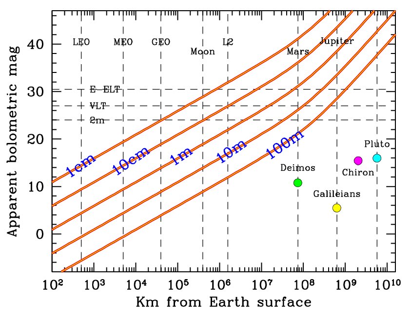
Figure 1 -
The apparent bolometric magnitude for man-made spacecraft at increasing distance
from Earth, according to eq. (2). Probe scale-size is labelled along each
curve. The altitude of LEO (set to 500 km), MEO (5000 km) and GEO terrestrial orbits is
marked, together with a few small bodies in the Solar System and their reference interplanetary
distances at Earth's opposition. The limiting magnitude reached by a 2m mid-class
telescope, the 8m ESO VLT and the forthcoming 40m E-ELT telescope, when observing distant Sun-type
stars, is also sketched on the plot.
|
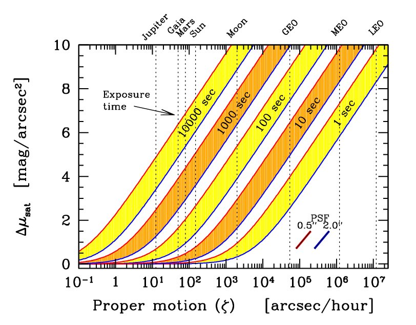
| Figure 2 -
The surface-brightness dimming for trailing satellites, according to
eq. (5). Different exposure times are assumed, as labelled. Each strip has a
lower and upper envelope for a 2" and 0.5" FWHM seeing figure,
respectively. The reference angular speed for satellites in LEO, MEO, and GEO (Veis 1963) is reported
together with the mean sky motion for other relevant solar bodies. In addition,
we also display the mean angular velocity of spacecraft Gaia, along its Halo L2
orbit.
|
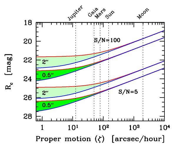 |
Figure 3 -
The magnitude limit reached by a 8m telescope, with a DQE = 0.8, at a 5 and 100 S/N
detection level in 100 (upper envelope) and 1000 sec (lower envelope of the curves) exposure time,
as from eq. (6).
We assume to observe in the Rc band under two extreme seeing conditions, namely
with a FWHM of 0.5 and 2.0 arcsec, and with a dark sky (μskyR = 20.5 mag
arcsec−2).
The indicative proper motion of some reference objects is reported, as from Fig. 2.
|
|
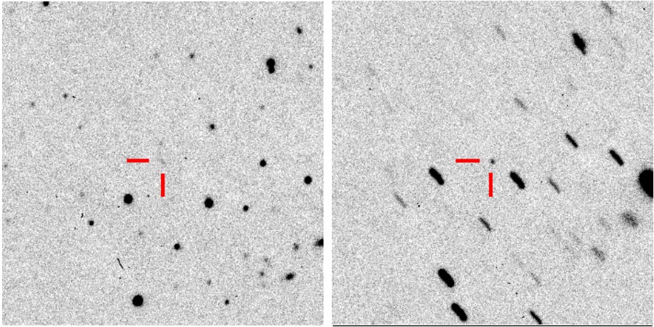
Figure 4 -
The spacecraft Gaia, as detected in the night of Oct 17-18, 2014 with the 1.52m
telescope of the Loiano Observatory. The two panels are consecutive 300 sec exposures
in "white" light (i.e. CCD with no photometric filter) of the same field with
sideral (upper) and differential (lower) telescope tracking on. The displayed field is 3×3 arcmin
across. North is up, East to the left. Pixel size is 0.58 arcsec. See text for a discussion.
|
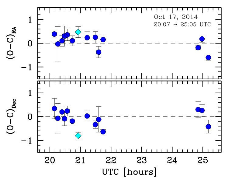 |
Figure 5 -
The angular residuals of Gaia's sky path along the night of Oct 17-18, 2014, as seen
from the Loiano Observatory (UAI observatory code "598"). The data of Table 1 are compared
with the corresponding JPL topocentric ephemeris. Residuals are in arcsec units, both for RA (upper panel)
and Dec (lower panel), in the sense "Observed−Computed", (O-C). The only sideral tracking observation
in our sample is singled out with a romb marker in both panels.
|
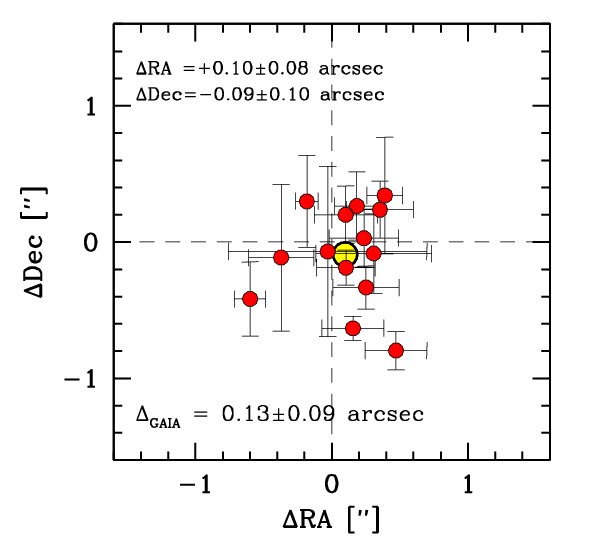 |
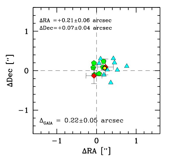
Figure 6 -
Arcsec coordinate residuals (in the sense "observed−computed") of the Gaia positions
along the night of Oct 17, 2014, with respect to the JPL topocentric ephemeris.
Mean RA and Dec offsets, together with their 1-σ uncertainty, are reported in the plot.
When combined, these lead to a mean path offset with respect to the nominal figure of
only ΔGAIA = 0.13 ± 0.09 arcsec (big circle in the plot).
|
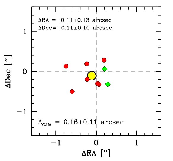 |
Figure 7 -
Same as Fig. 6 but for a set of astrometric measurements for the night of
Oct 14, 2014, taken with the 1.5m Mt. Lemmon (UAI code "G96") (Kowalski et al. 2014, dots)
and the 1.8m LPL/Spacewatch II (UAI code "291") telescopes Tubbiolo 2014, rombs).
Arcsec coordinate residuals are computed with respect to the correpsonding JPL topocentric ephemeris
leading to a mean orbital offset of ΔGAIA = 0.16 ± 0.11 arcsec (big circle in the plot).
|
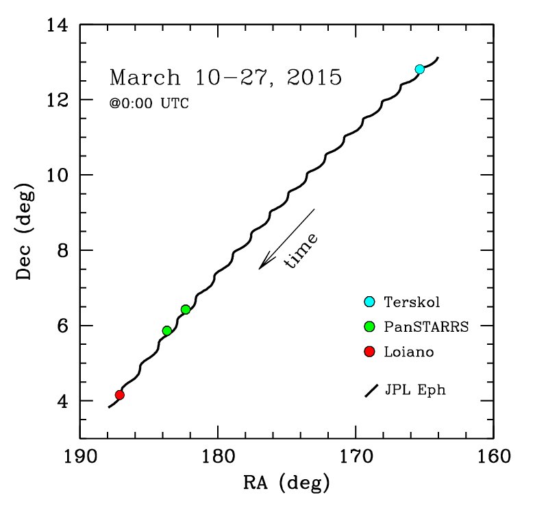 |
Figure 8 -
The Gaia sky path along the March 10-26, 2015 period.
The Terskol (UAI code "B18") (Velichko et al. 2015, cyan marker), PanSTARRS
(UAI code "F51") (Gibson et al. 2015, green dots) and Loiano (red dot) observations are
superposed to the JPL topocentric ephemeris (nominally for the B18 location, just as a guideline).
Note the daily "ripples" of the Gaia apparent orbit, due to the
parallax effect of Earth rotation, that superposes to the overall Lissajous figure on larger scales.
|
|
Figure 9 -
Same as Fig. 6 but for a coarser set of observations taken
during March 2015 at the Terskol 2m telescope (triangles), the 1.8m Pan-STARRS telescope (pentagons)
and the Loiano 1.52m telescope (rombs, see Table 1).
Arcsec coordinate residuals are computed with respect to the appropriate JPL topocentric ephemeris
for each observatory. Error bars are only available for our observations, as from Table 1.
The merged set of data leads to a mean orbital offset of
ΔGAIA = 0.22 ± 0.05 arcsec (yellow circle in the plot) along the spanned period.
|
|
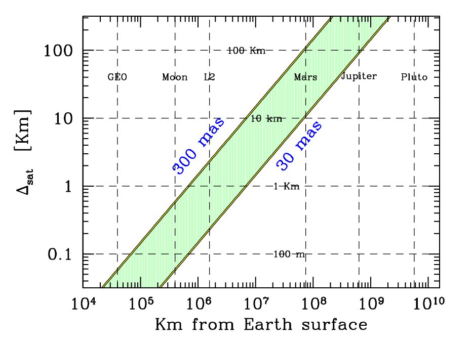
Figure 10 -
The expected spatial resolution in detecting distant spacecraft within the
Solar System. The transverse component, projected on the sky, is assessed in terms of
absolute resolution in kilometers at the different distances from Earth. Two representative
values for angular resolution of optical tracking are assumed, namely θmas = 300 mas
and 30 mas, as labelled on the plot.
|

|
Figure 11 -
The apparent magnitude of Gaia in different photometric bands along the
Oct 2014 and March 2015 observing runs.
In addition to Rc (dots) and V (square) Johnson-Cousins bands, "white"-light
(triangles) and Gunn z (romb marker) observations have been converted to the Rc magnitude
scale as discussed in the text. Dashed lines mark the mean Rc and V magnitude levels.
|
|
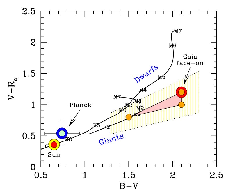
Figure 12 -
The Gaia color properties, as derived from the Grond reflectance curves of
Altmann et al. (2014), are assessed in the (B−V) vs. (V−Rc) plane. The spacecraft
location is compared with the stellar locus for dwarf and giant stars of different spectral type (as
labelled on the plot), according to Pecaut & Mamajek (2013) and
and Houdashelt et al. (2000), respectively. The shaded triangular region on the plot edges
the allowed color range of Gaia (including the experimented "face-on" orientation, as
discussed in the text), accounting for the reported variability of the spacecraft reflectance.
As a reference, the Sun is also marked on the plot, together with the derived colors of the
Planck probe, according to Altmann et al. (2014).
|
|
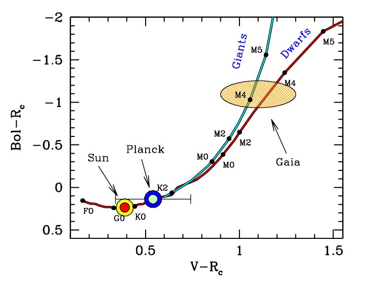
Figure 13 -
The observed Gaia (V−Rc) color is contrasted in the plot to constrain the
spacecraft bolometric correction. As for Fig. 12, the spacecraft location is compared
with the stellar locus for dwarf and giant stars of different spectral type (as labelled on
the plot), according to Pecaut & Mamajek (2013) and Houdashelt et al. (2000), respectively, and
with the relevant points for the Sun and Planck probe.
|
|
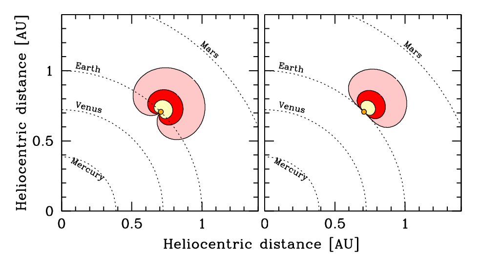
Figure 14 -
Visibility maps of deep-space probes, as optically tracked from Earth with
1hr CCD exposure by different telescopes.
Sky conditions assume a seeing FWHM = 1 arcsec and
μskyR = 20.5 mag arcsec−2.
The Gaia effective area A = 105 cm2 (that is by assuming α = 0.11
as a conservative estimate of the true Bond albedo) has been taken as a reference.
The marked "horizons" in all panels assume to observe with a 2m (yellow region),
8m (red), and 40m (pink) telescopes, at (S/N)>5 detection
threshold. The small orange dot marks Earth's influence sphere
(edging the Lagrangian L1 and L2 points), throughout.
Left panel refers to the case of a spherical spacecraft, while right panel
assumes a prevailing planar structure of the target. Mercury, Venus, Earth, and Mars
orbits are sketched, as a guideline.
|
|
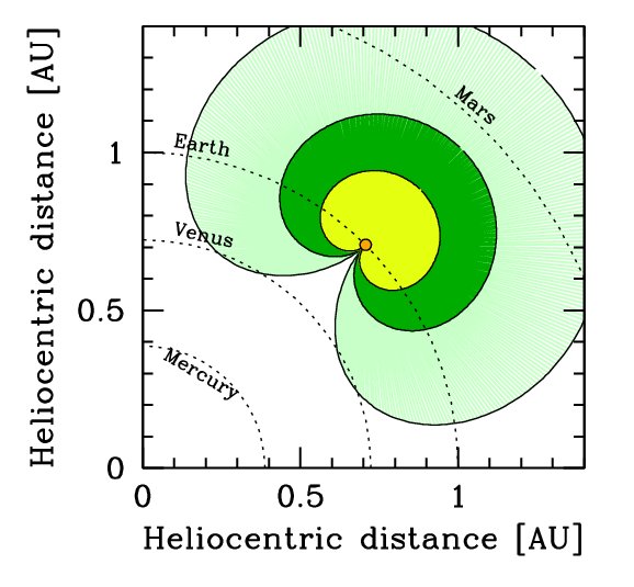
Figure 15 -
Same as Fig. 14 but for 2m (green), 8m (dark green) and 40m (pale green)
telescopes looking (at a S/N ~ 5 or better threshold) at a deep-space spherical probe of
Gaia's 10× enhanced effective area (namely A = 106 cm2).
Under these more favourable circumstances, note that a VLT-class telescope could yet
confidently track a spacecraft along most of its Hohmann trajectory to Mars and Venus,
while a 2m telescope could, in general, effectively probe distant spacecraft
some 40 million km away from Earth.
|
Back to article listing |
|
Shortcut to Space Stuff |
| AB/May 2017 |
|
|