Back to article listing

Back to article listing |
|
Shortcut to Space Stuff |
| Annibali, F., Tosi, M., Romano, D., Buzzoni, A., Cusano, F., Fumana, M., Marchetti, A., Mignoli, M., Pasquali, A., Aloisi, A.: |
| "Planetary Nebulae and HII Regions in the Starburst Irregular Galaxy NGC 4449
from LBT MODS Data", 2017, The Astrophysical Journal, 843, 20 |
|
|
Summary:
We present deep 3500-10000 Å spectra of HII regions and planetary nebulae (PNe)
in the starburst irregular galaxy NGC 4449, acquired with the Multi Object Double
Spectrograph at the Large Binocular Telescope. Using the "direct" method, we derived
the abundance of He, N, O, Ne, Ar, and S in six HII regions and in four PNe in NGC 4449.
This is the first case of PNe studied in a starburst irregular outside the Local Group.
Our HII region and PN sample extends over a galacto-centric distance range of ~2 kpc
and spans ~0.2 dex in oxygen abundance, with average values of 12+log(O/H)=8.37 ± 0.05
and 8.3 ± 0.1 for HII regions and PNe, respectively. PNe and HII regions exhibit similar
oxygen abundances in the galacto-centric distance range of overlap, while PNe appear
more than ~1 dex enhanced in nitrogen with respect to HII regions. The latter result is
the natural consequence of N being mostly synthesized in intermediate-mass stars and
brought to the stellar surface during dredge-up episodes. On the other hand, the similarity
in O abundance between HII regions and PNe suggests that NGC 4449's interstellar medium has
been poorly enriched in a elements since the progenitors of the PNe were formed. Finally,
our data reveal the presence of a negative oxygen gradient for both H II regions and PNe,
whilst nitrogen does not exhibit any significant radial trend. We ascribe the (unexpected)
nitrogen behaviour as due to local N enrichment by the conspicuous Wolf-Rayet population
in NGC 4449.
|
| Pick up the paper at Astro-ph/1706.02108 | Local link to the PDF version (1.8 Mb) | ||
|
Enhanced HTML/PDF version at the ApJ site (*) (*) May require access password |
|
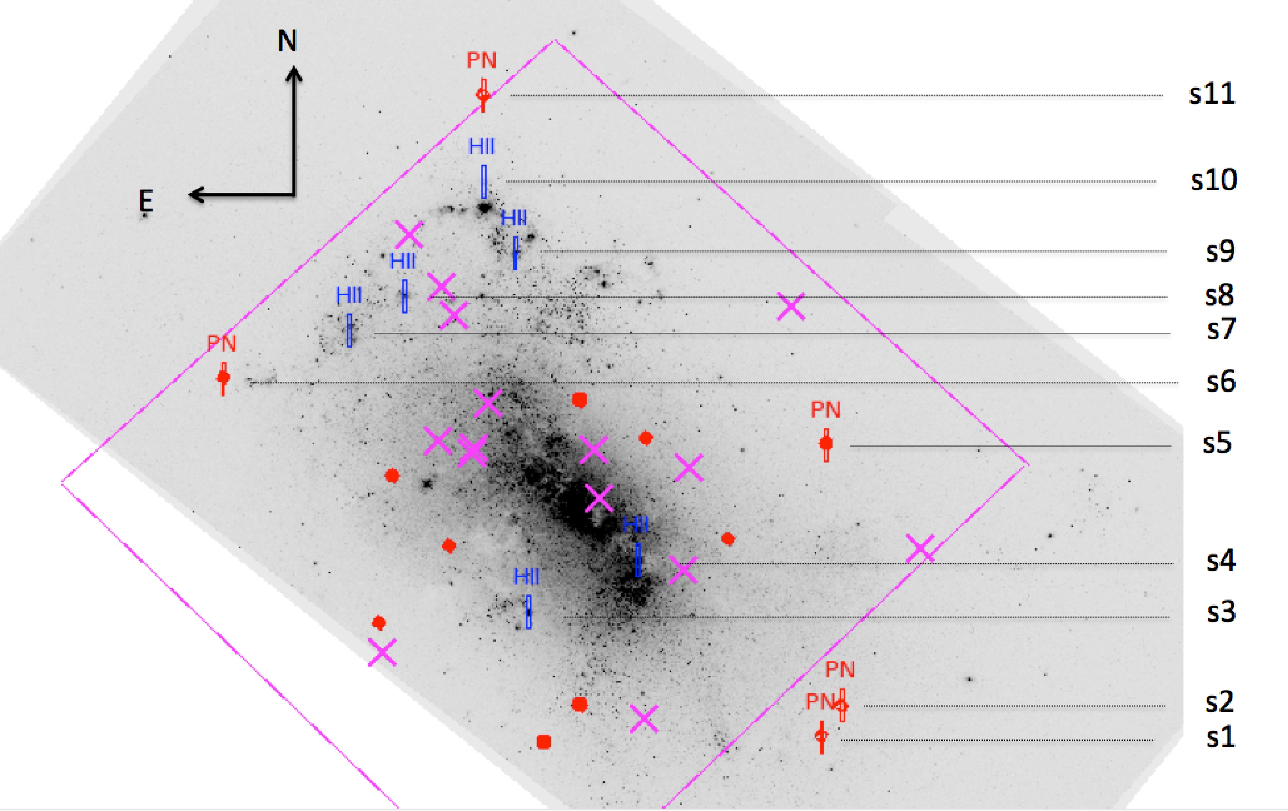
Figure 1 -
HST/ACS image of NGC 4449 in F555W (~V) with superimposed our HII region and PN sample. The smaller
field of view covered by the ACS F502N (~[OIII]) image is also indicated with the magenta line. The small
red points and magenta crosses indicate the totality of the 28 PNe identified from the combined
F435W (~B)-F502N-F814W (I) image, and then cross-checked in F658N (Hα). The small red points
denote the 13 PNe also identified when using the combined B, V, I image. Superimposed on the image
are the eleven LBT/MODS 1"x10" slits at the position of the 6 HII regions and 5 PNe targeted for spectroscopy.
|
|
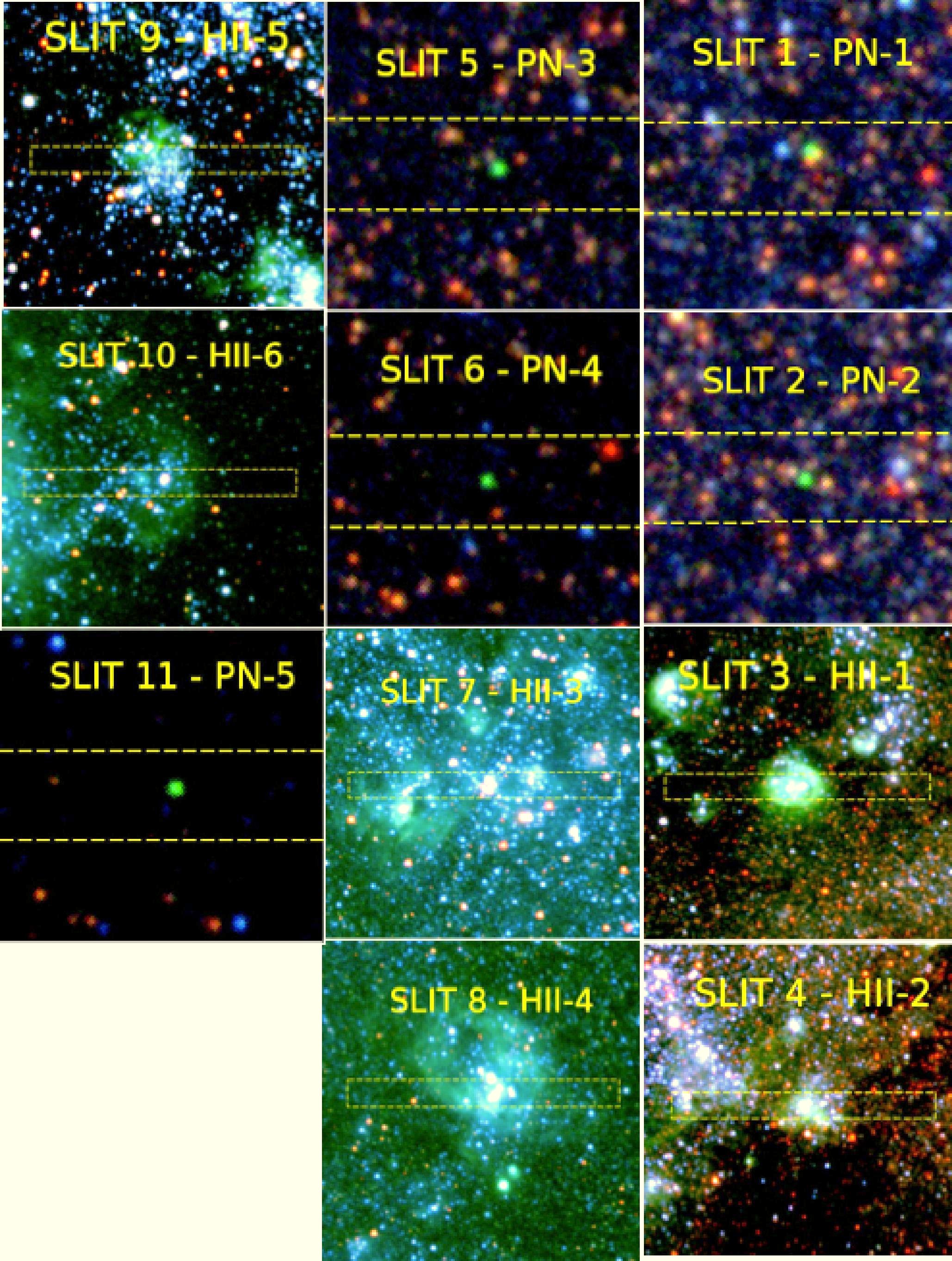
| Figure 2 -
HST/ACS color-combined images (F435W=blue, F555W=green, F814W=red) of PNe and HII regions in NGC 4449
targeted for spectroscopy with LBT/MODS. The FoV shown is ~3.5"x3.5" for the PNe and 12"x12" for the HII regions.
|
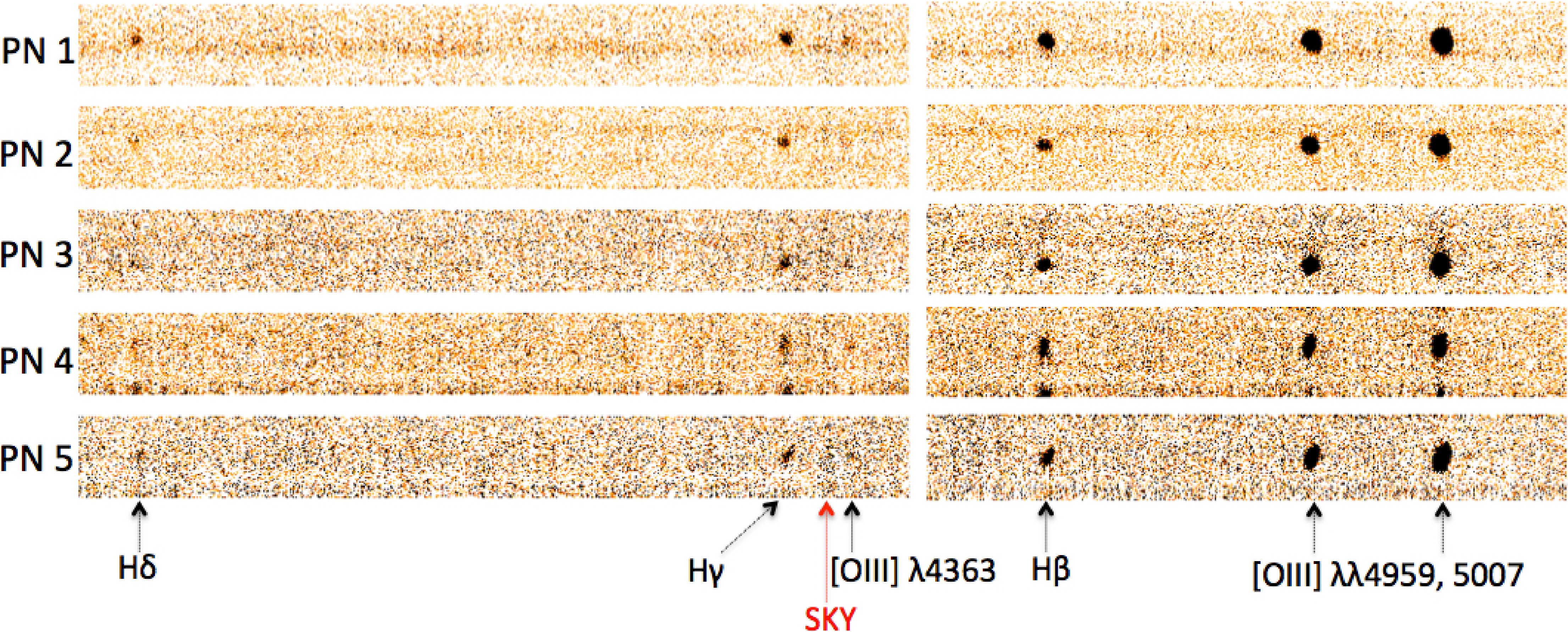 |
Figure 3 -
Two-dimensional MODS spectra of PNe in NGC 4449 showing the Hδ, Hγ, [OIII]λ4363,
Hβ and [OIII]λλ4959, 5007 lines. The residuals corresponding to the subtraction of the
HgIλ4358 sky line, between the Hγ and [OIII]λ4363 lines, are visible in the 2D spectra.
|
|
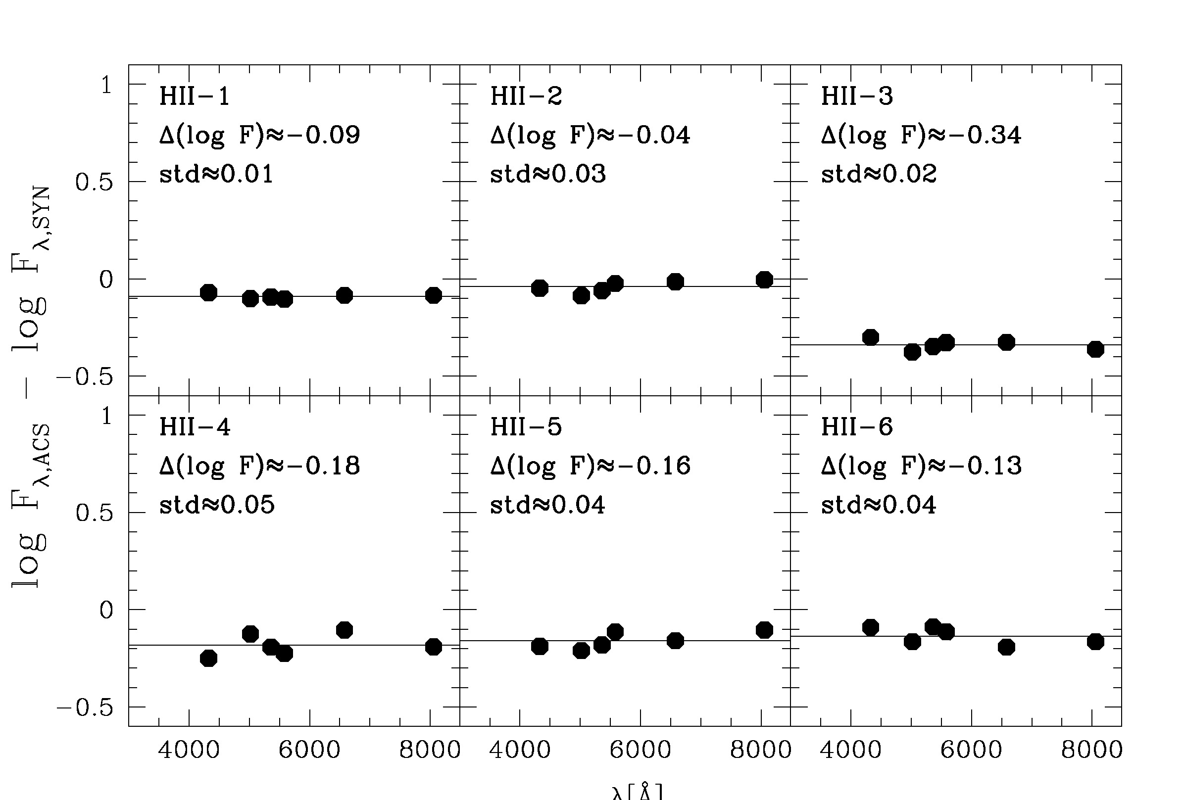
Figure 4 -
Comparison between ACS and Synphot fluxes for HII regions in NGC 4449 (see Section 2).
From blue to red wavelengths, the dots correspond to the following ACS bandpasses: F435W, F502N, F555W,
F550M, F658N and F814W. For each HII region, the solid horizontal line is the average
log(Fλ,ACS) − log(Fλ,SYN) offset.
The standard deviation around this value is also indicated within each panel.
|
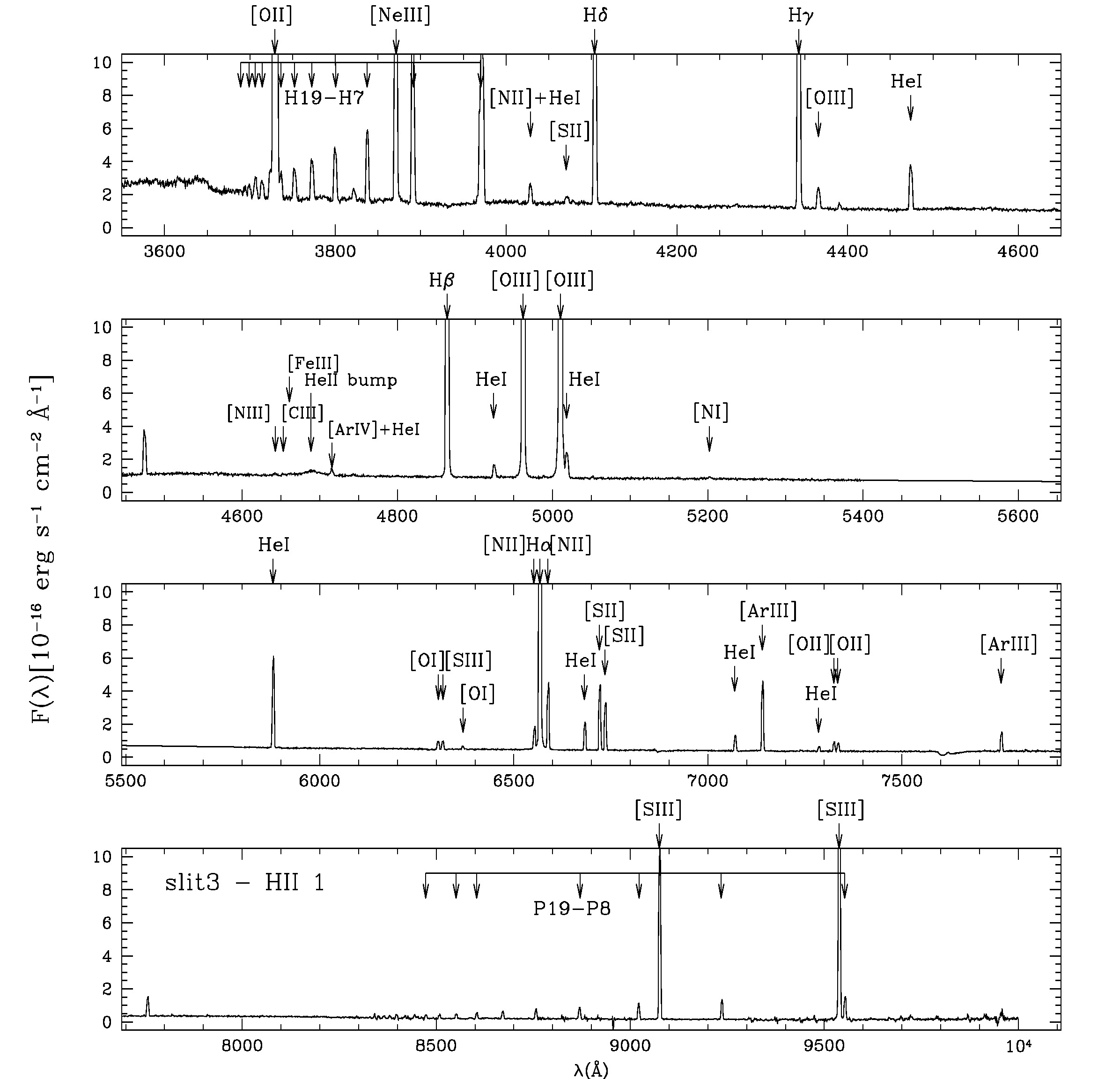 |
Figure 5 -
LBT/MODS spectra in the blue and red channels for HII-1 in NGC 4449 with indicated all the identified
emission lines. A linear interpolation was performed in the 5400-5800 Å region where the
sensitivities of the blue and red detectors drop. The spectra of the other HII regions
(HII-2, HII-3, HII-4, HII-5, HII-6) are provided in the Appendix.
|
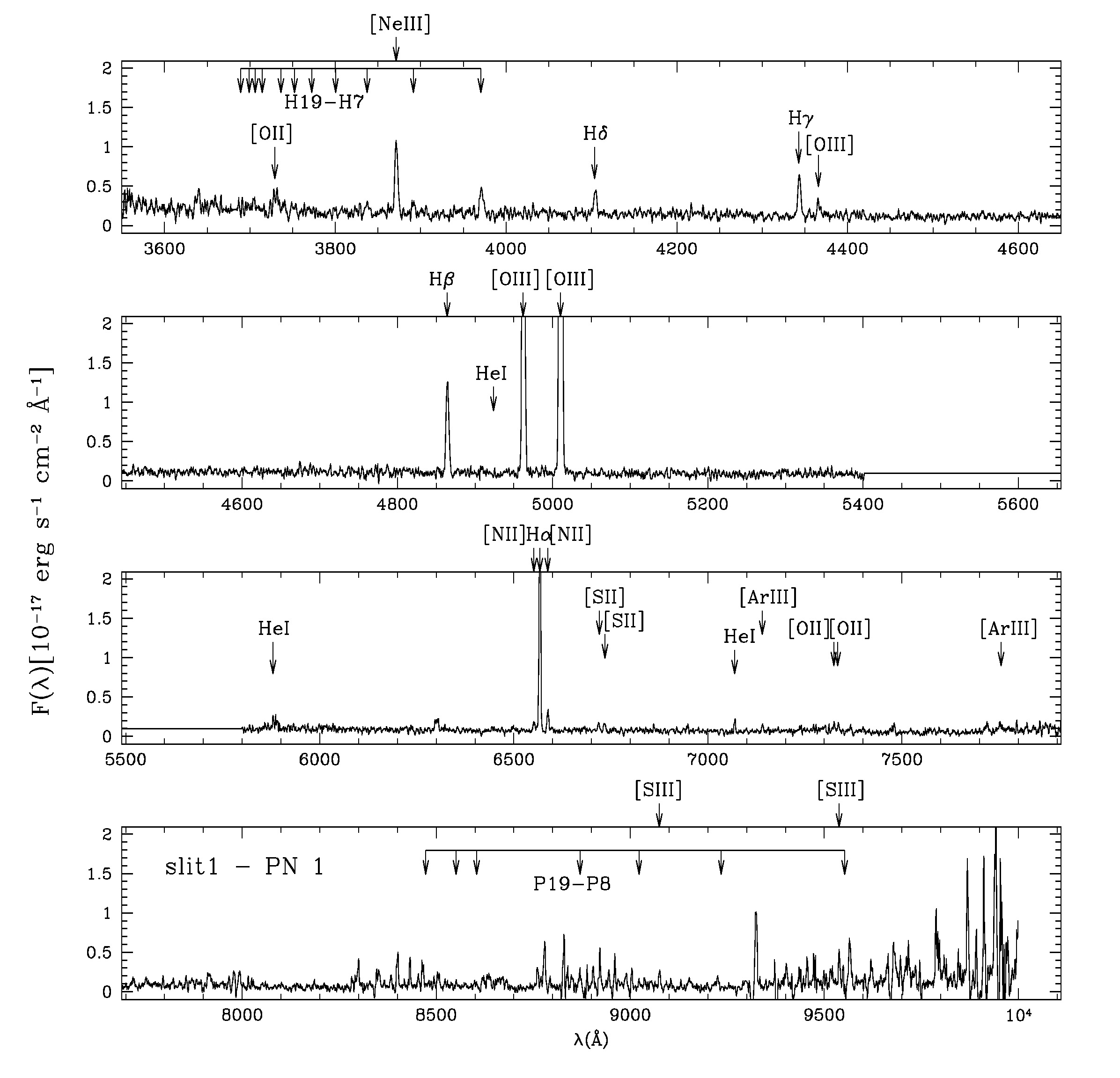 |
Figure 6 -
LBT/MODS spectra in the blue and red channels for PN-1 in NGC 4449 with indicated all the identified
emission lines. A linear interpolation was performed in the 5400-5800 Å region where the
sensitivities of the blue and red detectors drop. A ~1 Å boxcar filter smoothing was applied
to the spectrum to better highlight the low signal-to-noise features.
The spectra of the other PNe (PN-2, PN-3, PN-4, PN-5) are provided in the Appendix.
|
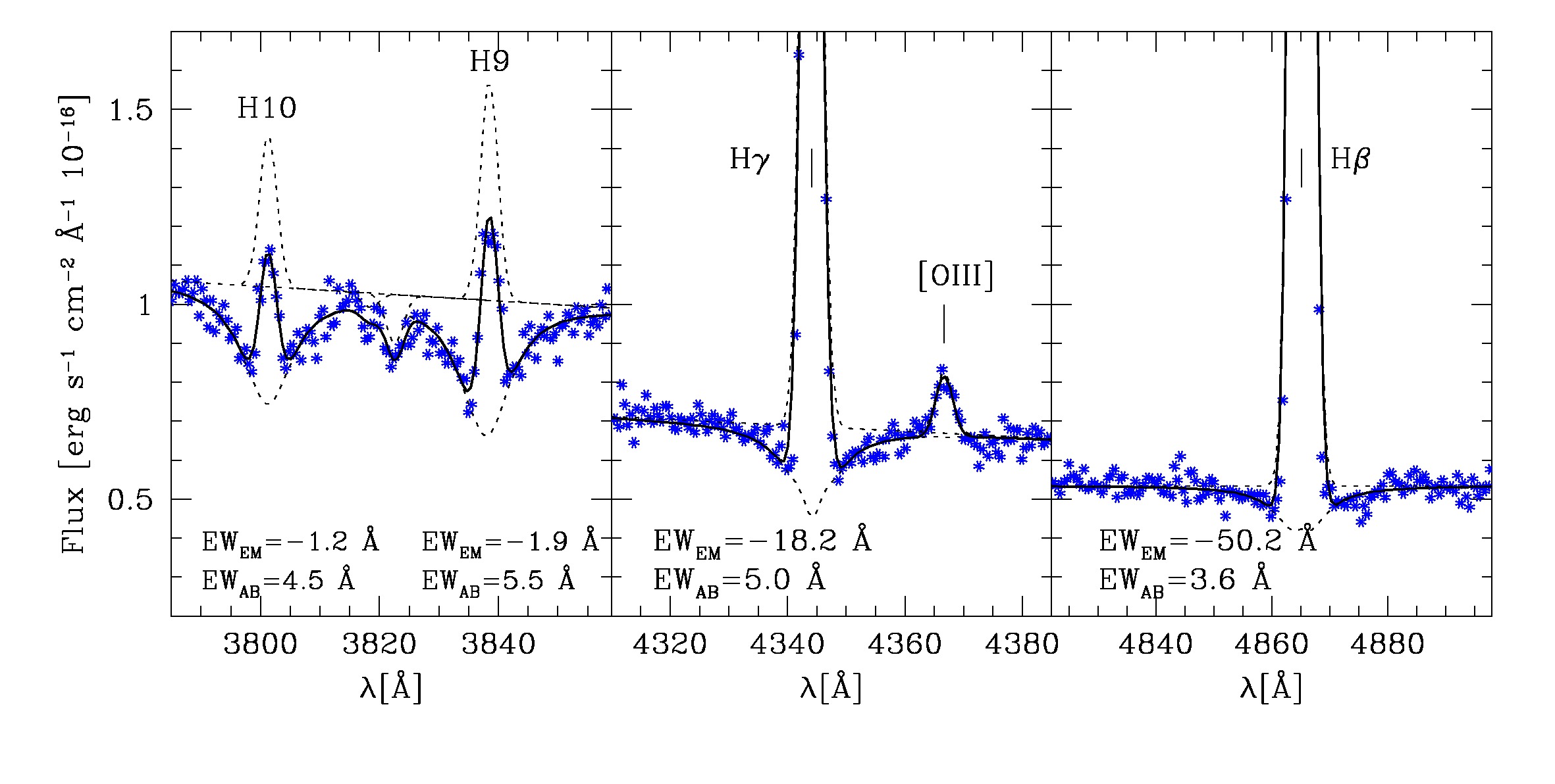 |
Figure 7 -
Example (region HII-6) of spectral fit to the regions around some Balmer lines. The asterisks are the
observed spectrum, while the continuous line is the best fit. The individual components of the fit are
plotted with a dashed line: linear continuum, Gaussian profiles for the emission lines, and Voigt profiles
for the Balmer absorption lines.
The outcome of fit to the H10(λ3798) and H9(λ3835) lines, with prominent absorption wings,
was used to fix the Lorentian and Gaussian FWHMs during the fit to redder Balmer lines. The derived Balmer
equivalent widths in absorption and in emission are provided within each panel. The absorption feature
between H10 and H9 is due to a blend of FeI lines.
The figure clearly shows that the contribution of absorption with respect to emission becomes increasingly
lower toward redder wavelengths (see section 3.1 for more details.)
|
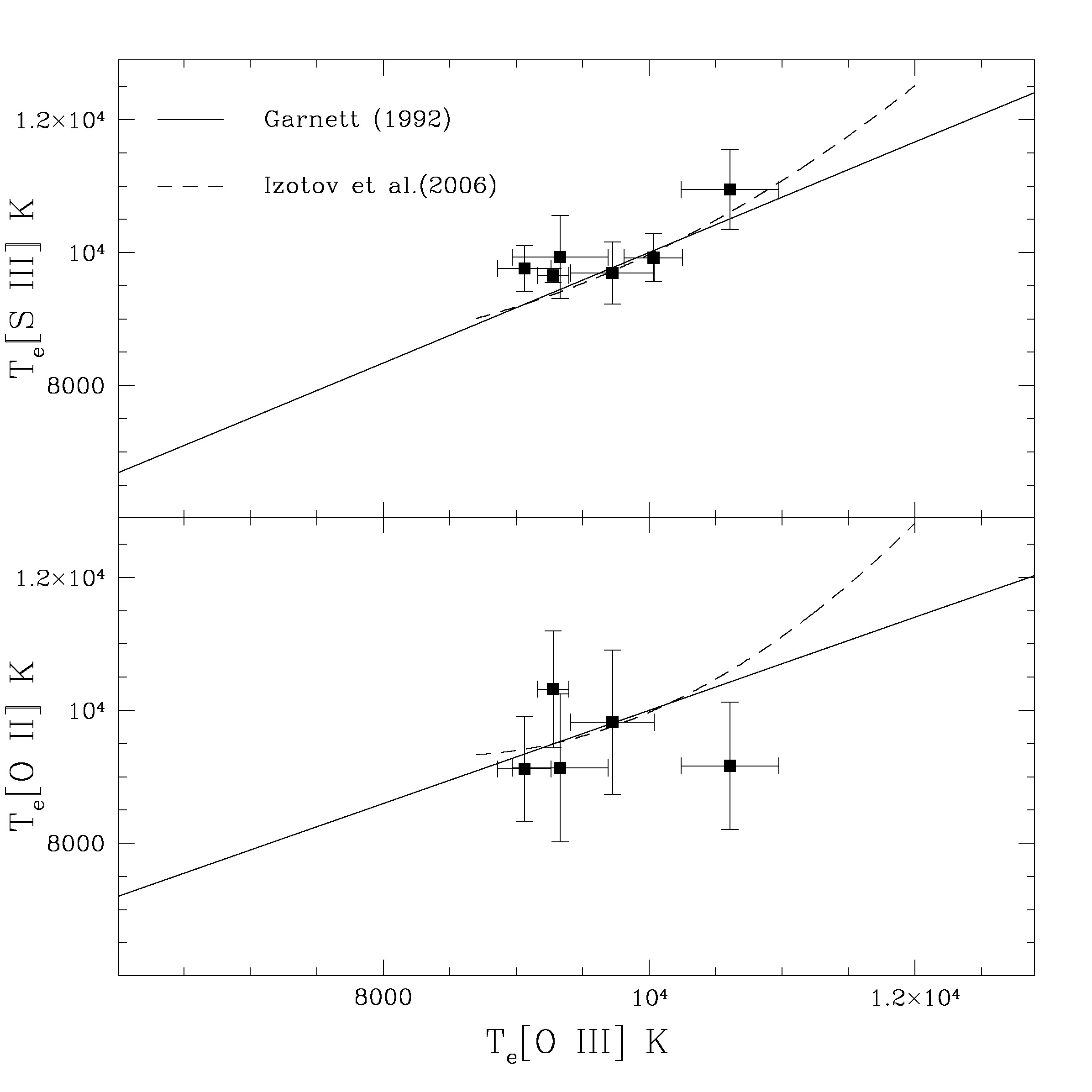 |
Figure 8 -
Correlations between electron temperatures derived for HII regions in NGC 4449 through different
diagnostics: [OIII]λ4363/[OIII]λλ4959,5007 for Te[OIII],
[SIII]λ6312/[SIII]λλ9069,9532 for Te[SIII], and
[OII]λλ3726,29/[OII]λλ7320,30 for Te[OII].
The solid and dashed lines are the predicted correlations based on photoionization models
from Garnett (1992) and from Izotov et al. (2006), respectively.
|
|
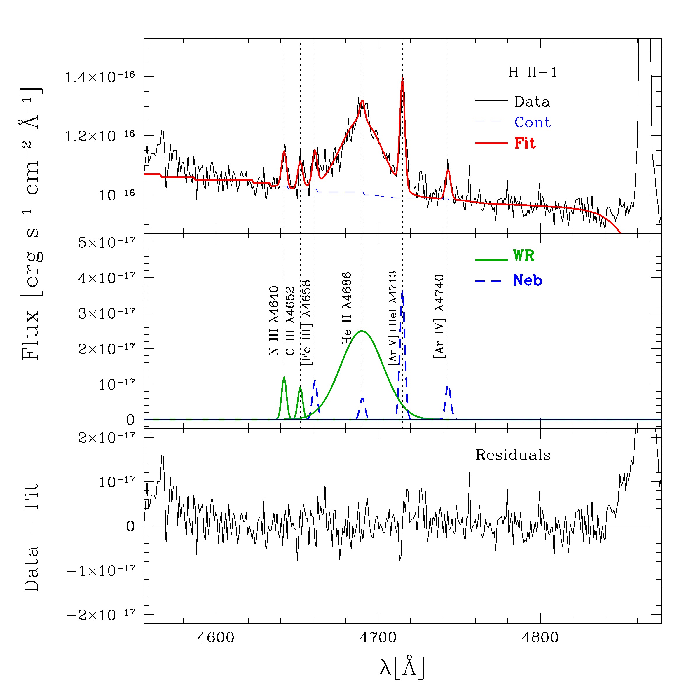
Figure 9 -
Portion of the spectrum of HII-1 around the region of the Wolf-Rayet blue bump at ~4690 Å.
Top panel: Observed spectrum (thin black line) and total (continuum plus emission lines) fit
(red thick line). The continuum has been modelled with a Z=0.004, 3-4 Myr old SSP, normalized at
4770-4840 Å (see Section 5 for details).
Middle panel: fitted emission lines (solid green line for WR features, dashed blue line for
nebular narrow emission lines). Bottom panel: residual after subtracting the best-fit model.
|
|
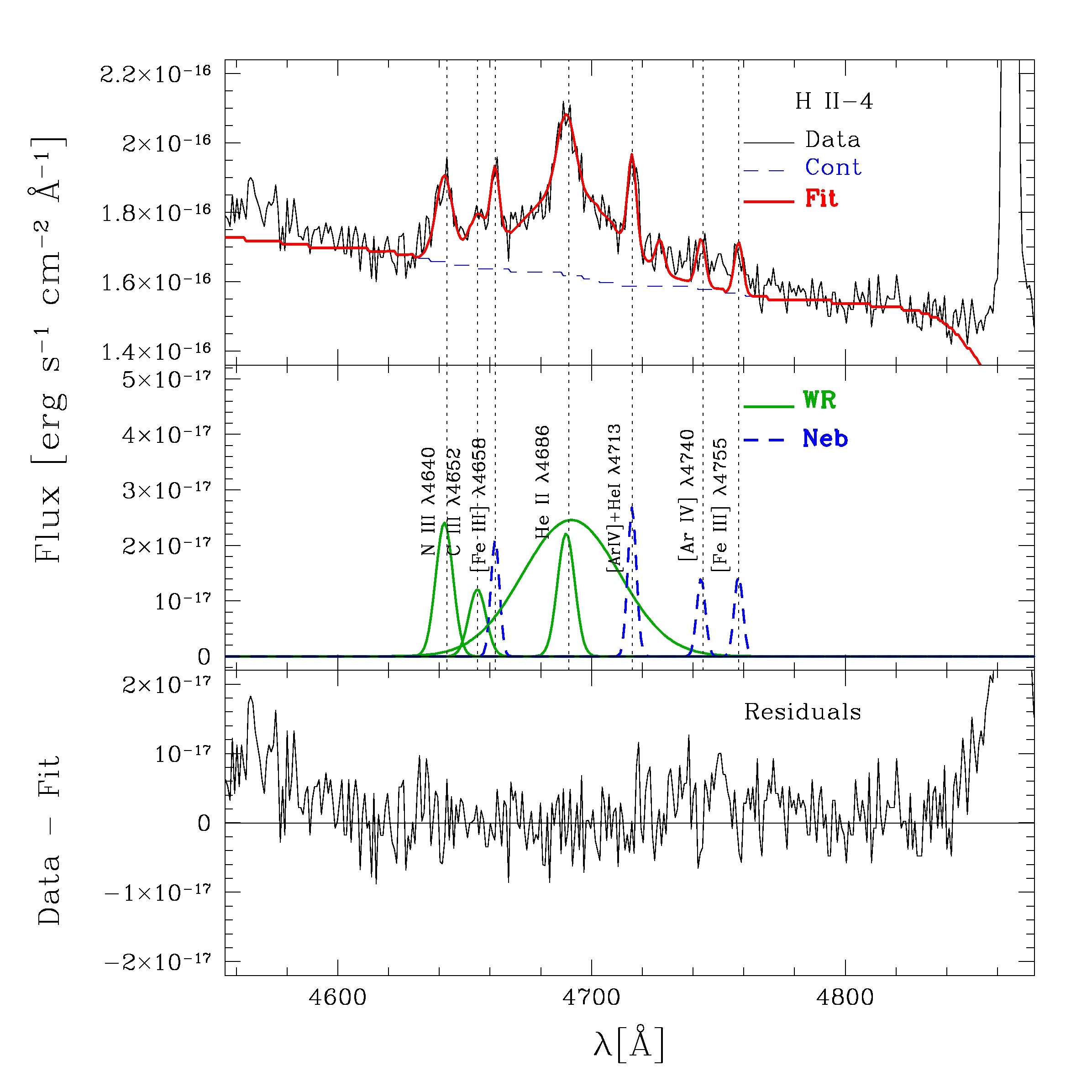
Figure 10 -
Same as in Figure 9 but for HII-4.
|
|
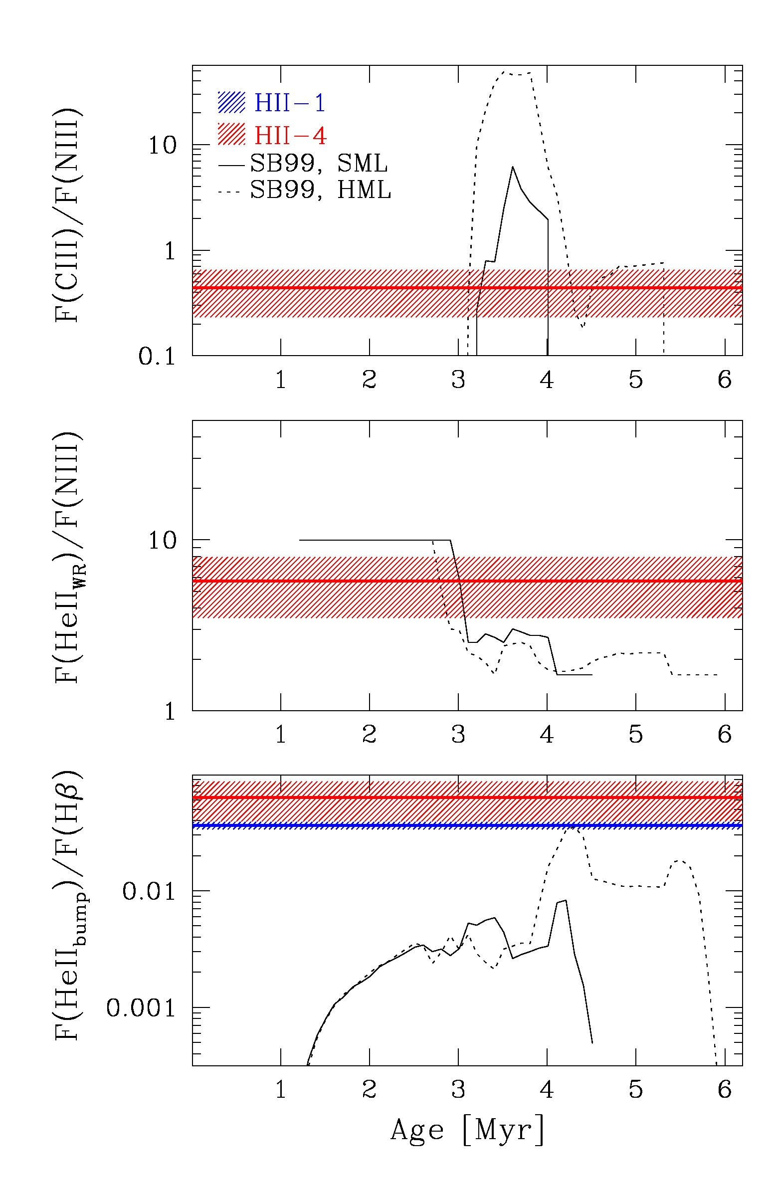
Figure 11 -
Wolf-Rayet features detected in regions HII-1 and HII-4 against Starburst99 (SB99) models. The models
are based on the Geneva tracks with metallicity Z=0.008 with a standard mass-loss prescription (solid line)
and with a high mass-loss prescription (dotted line). From top to bottom: F(CIII)/F(NIII),
F(HeIIWR)/F(NIII), and F(HeIIWR)/F(Hβ) ratios versus age. Notice that the
F(HeIIWR) flux refers to the broad WR component without the contribution from the nebular HeII
emission line.
|
|
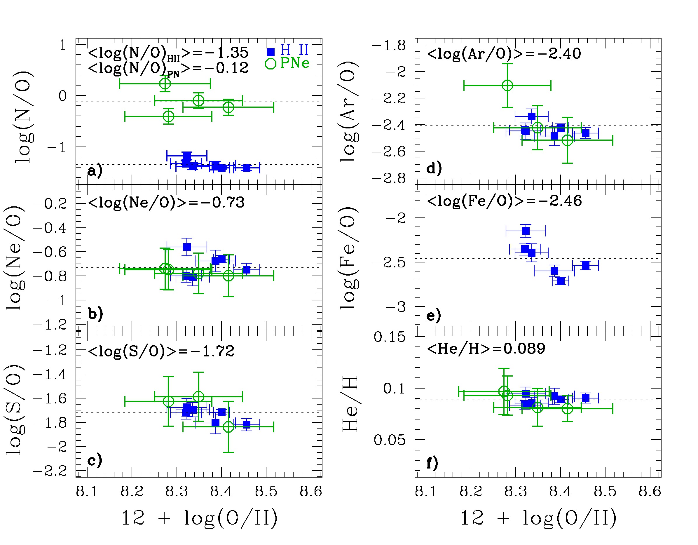
Figure 12 -
Abundance ratios as a function of total oxygen abundance. Solid and open symbols are for HII regions and PNe,
respectively. Within each panel, the label and the dotted horizontal line indicate the average value for the
combined HII region and PN data; only in panel a), separate log(N/O) mean values for HII regions and PNe
are provided.
|
|
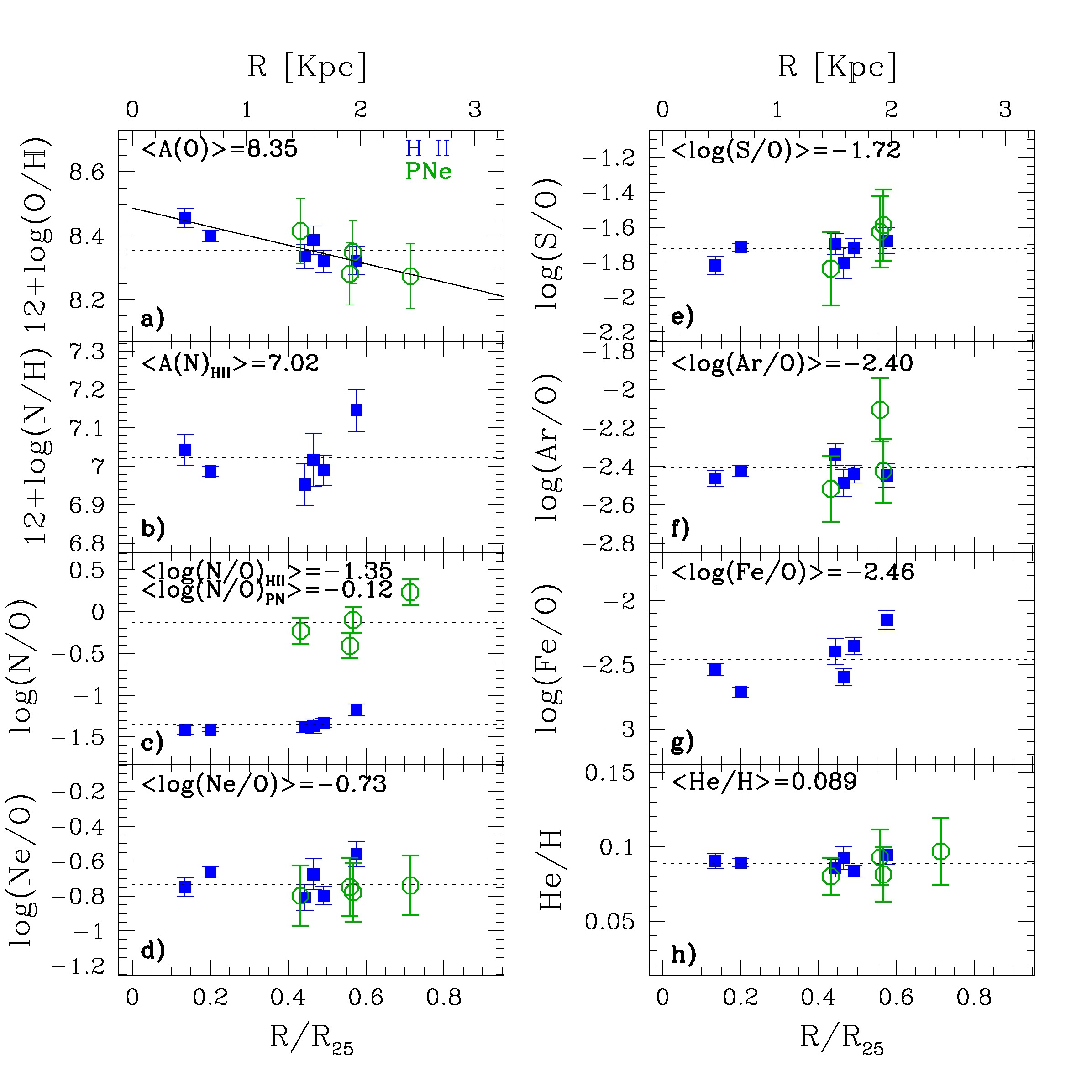
Figure 13 -
Element abundances and abundance ratios as a function of galacto-centric distance R/R25, where
R25=3.4 kpc. The linear galacto-centric scale in kpc is also indicated on top. Solid and
open symbols are for HII regions and PNe, respectively. Within each panel, the label and the dotted
horizontal line indicate the average value for the combined H~II region and PN data; only in panel c),
separate log(N/O) mean values for HII regions and PNe are provided. In panel b), in order to better
visualise the range of nitrogen variation as a function of radius for HII regions, we do not include
PNe, whose N abundance is so high (see Table 8) that the ordinate scale would be too compressed.
|
|
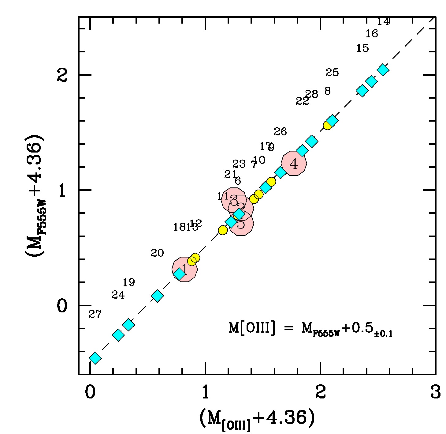
Figure 14 -
The MF555W magnitudes of the spectroscopic PN sample are compared to the corresponding
M[OIII] values (big dot markers).
All magnitudes have been corrected for the distance modulus and offset by a
value of +4.36 mag, corresponding to the PNLF bright cutoff magnitude (M*[OIII]).
A straight relationship is in place with M[OIII]−MF555W = 0.5±0.1.
When applied to the total photometric PN sample
(diamond markers), this offset allows us to assess the M[OIII] distribution
of the whole sample of 28 PNe showing that our observations actually probed the bright
tail of NGC 4449 PNLF, down to (M[OIII]−M*[OIII])~2.5 mag.
In the plot each nebula is labeled according to its entry ID of Table 9.
|
|
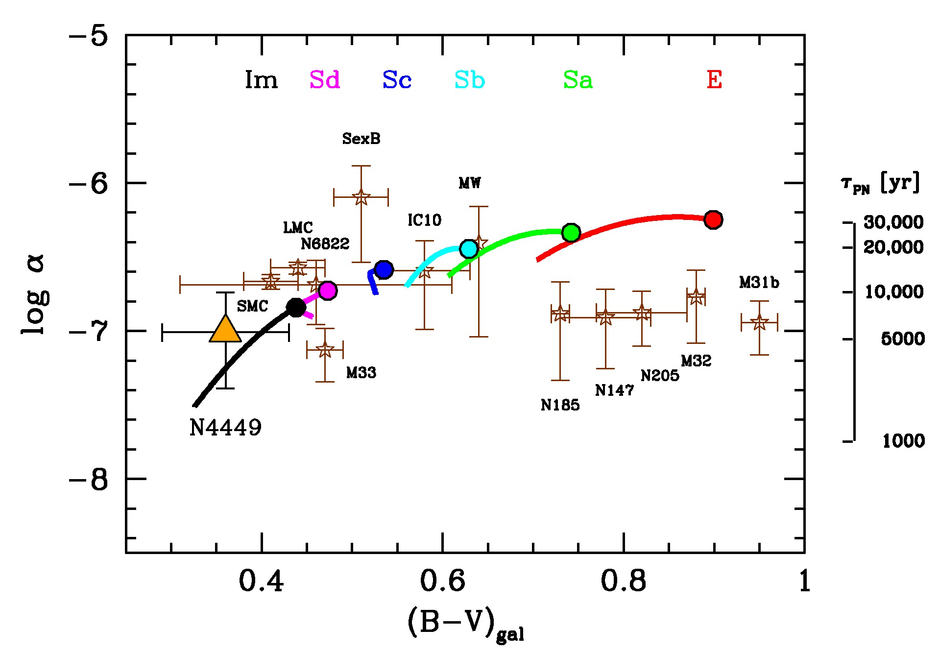
Figure 15 -
A comprehensive overview of the derived luminosity-specific PN number density
α for NGC 4449, compared with Local Group galaxies (star markers) as from Buzzoni et al. (2006).
Also superposed are the Buzzoni (2005) template galaxy models along the whole morphological sequence from 2
to 15 Gyr, with the latter limit marked by the big solid dots. The Weidemann (2000) empirical scheme
is adopted for properly assessing stellar mass loss in the galaxy models. An indicative estimate of the
mean representative PN visibility timescale (in years) is sketched on the right scale, as discussed in the text.
|
|
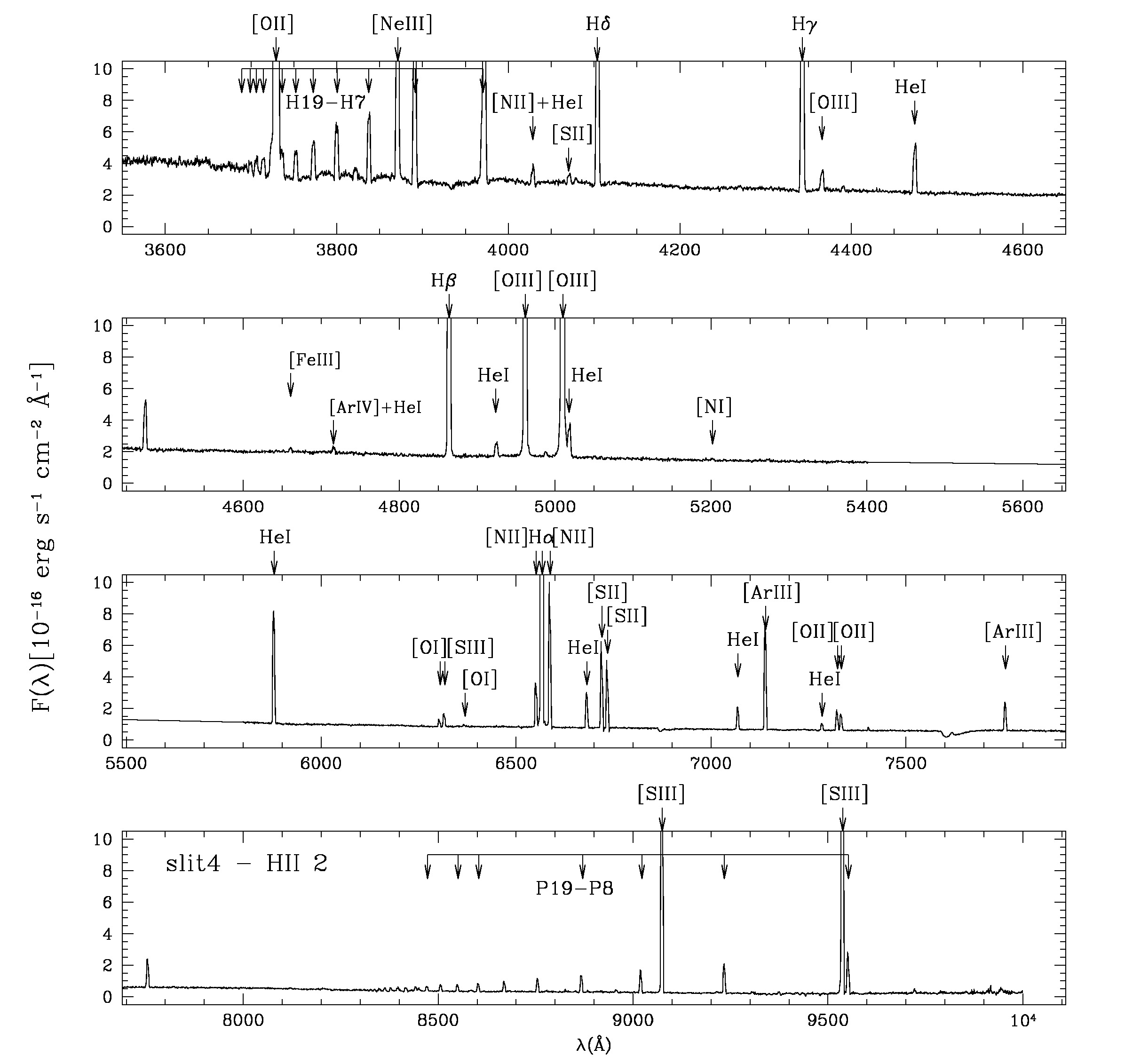
Figure 16 -
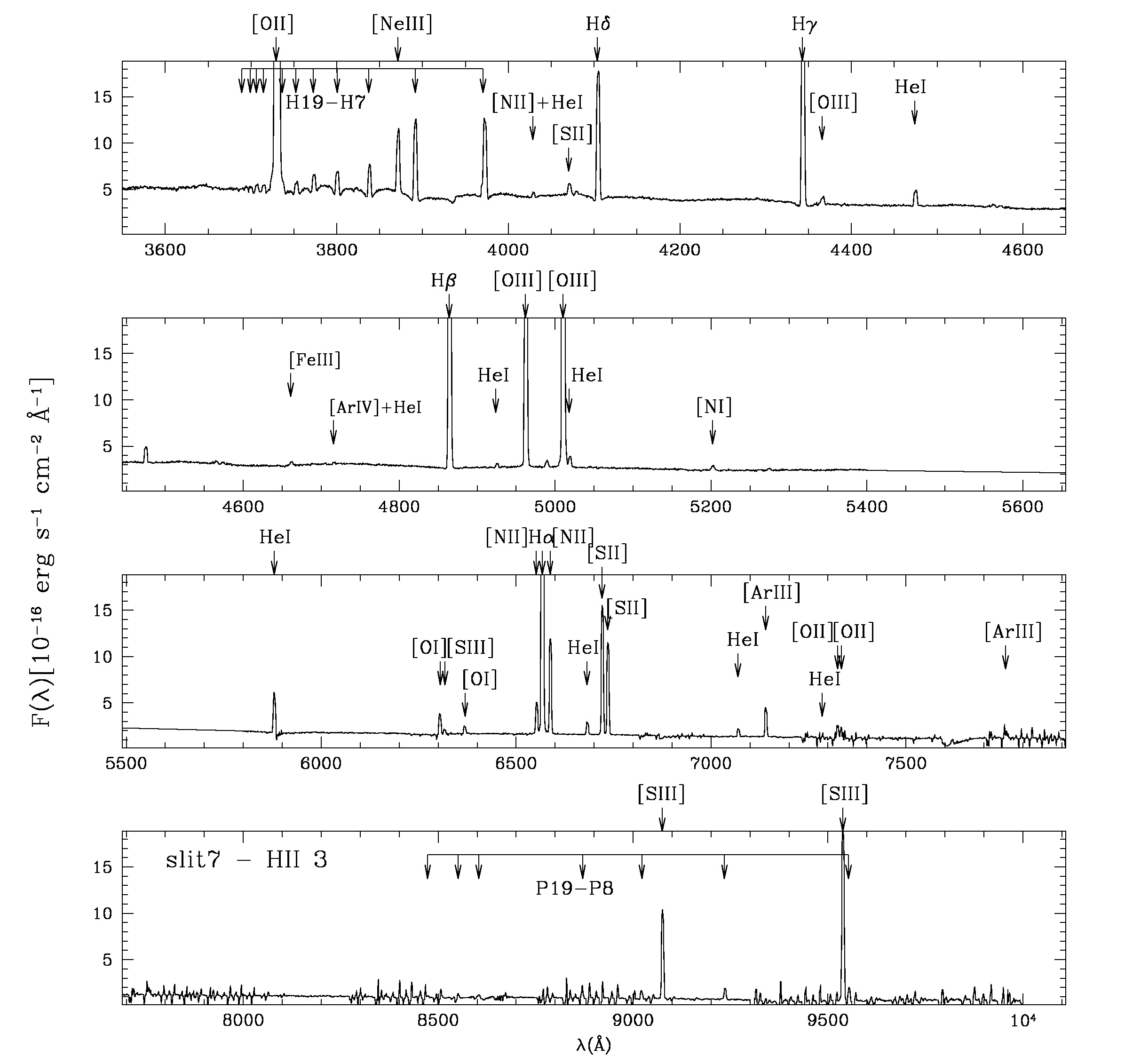
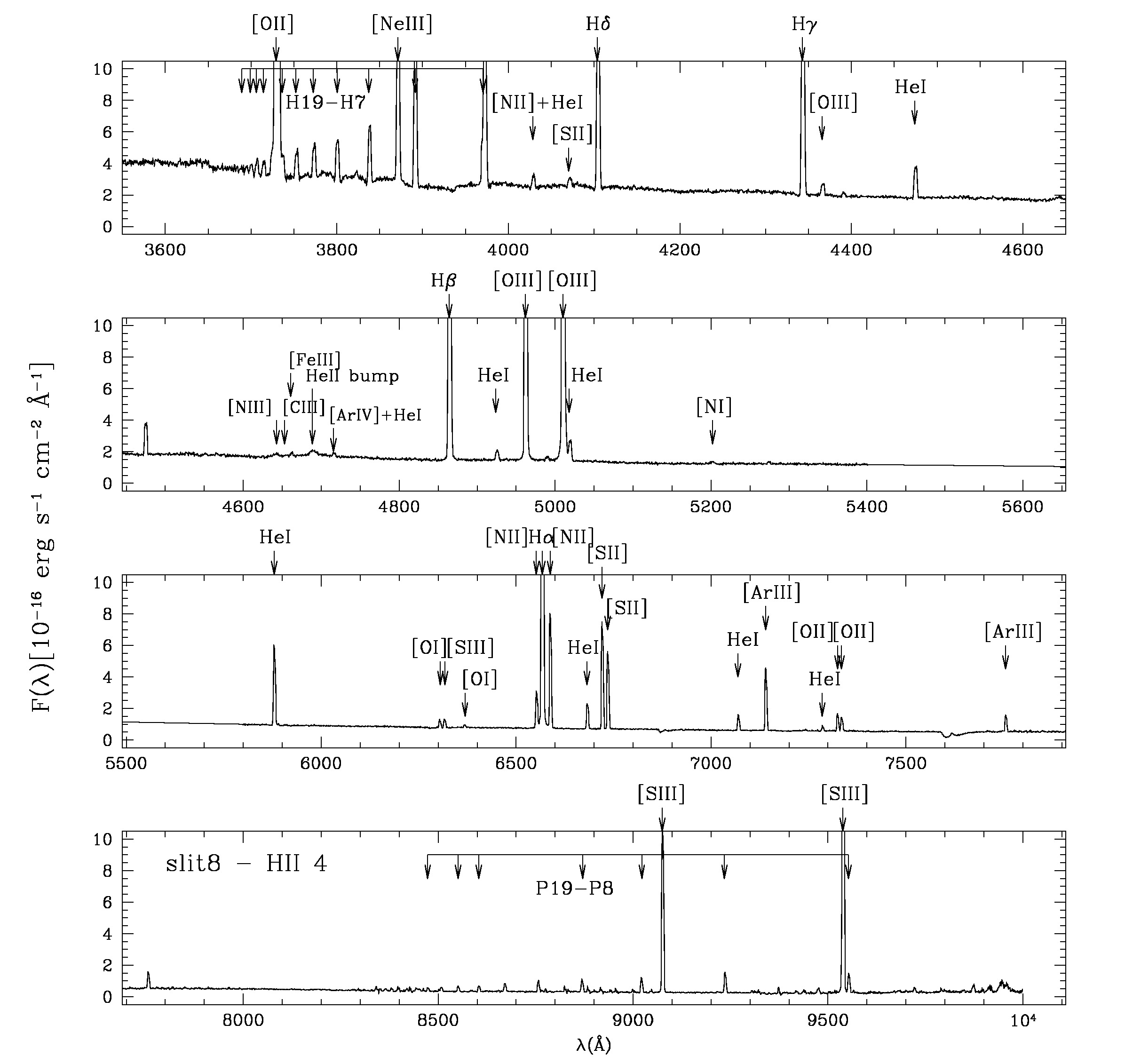
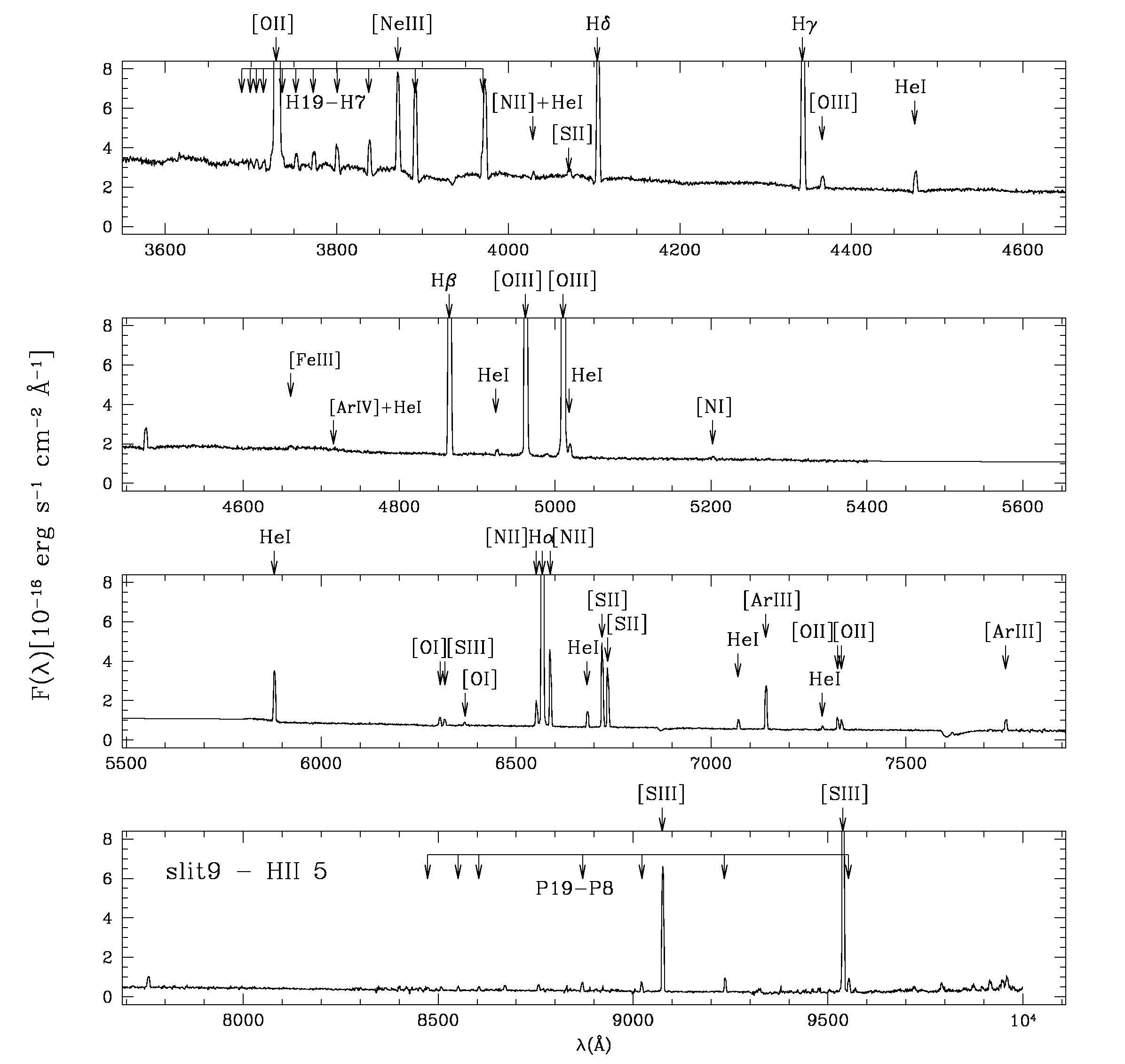
LBT/MODS spectra in the blue and red channels for HII-2 in NGC 4449 with indicated all the identified
emission lines. The spectra have been scaled such that the details are evident.
|
|
Figure 17 -
Same as Fig. 16 but for HII-3.
|
|
Figure 18 -
Same as Fig. 16 but for HII-4.
|
|
Figure 19 -
Same as Fig. 16 but for HII-5.
|
|
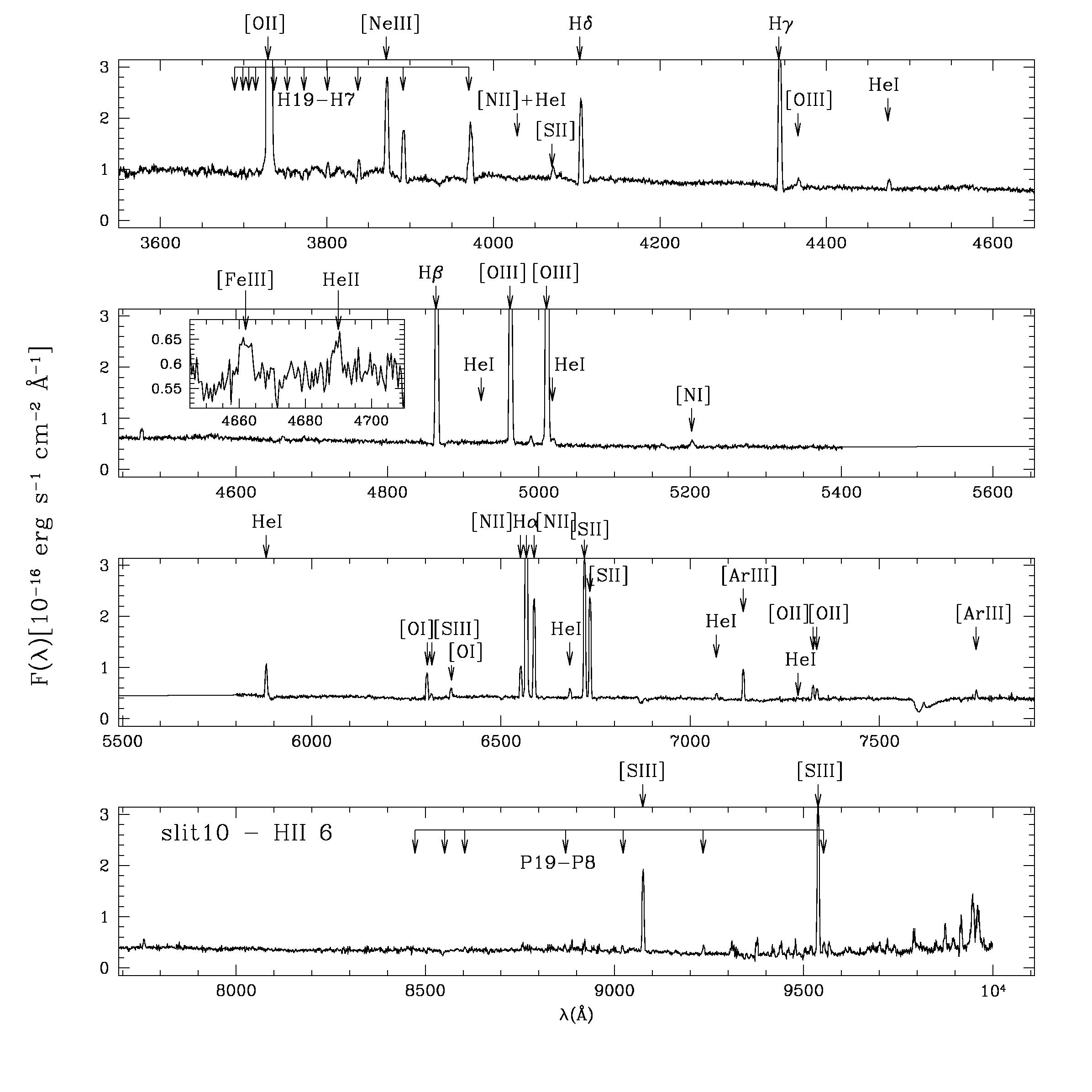
Figure 20 -
Same as Fig. 16 but for HII-6. The small insertion provides a zoom into the ~4640-4710Å wavelength
range to highlight the faint [FeIII]λ4658 and HeIIλ4686 lines.
|
|
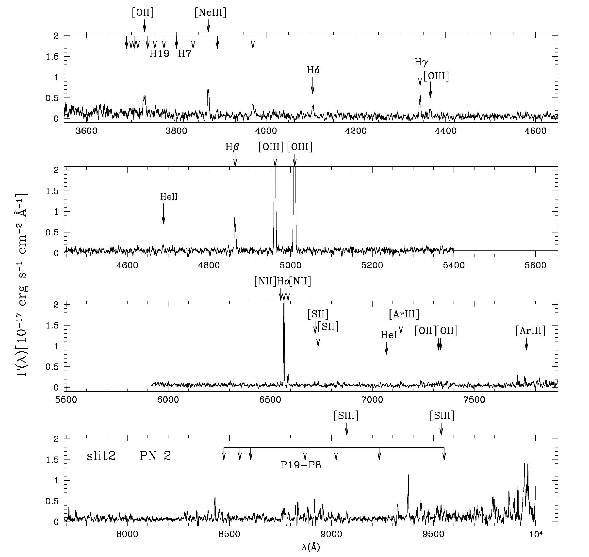
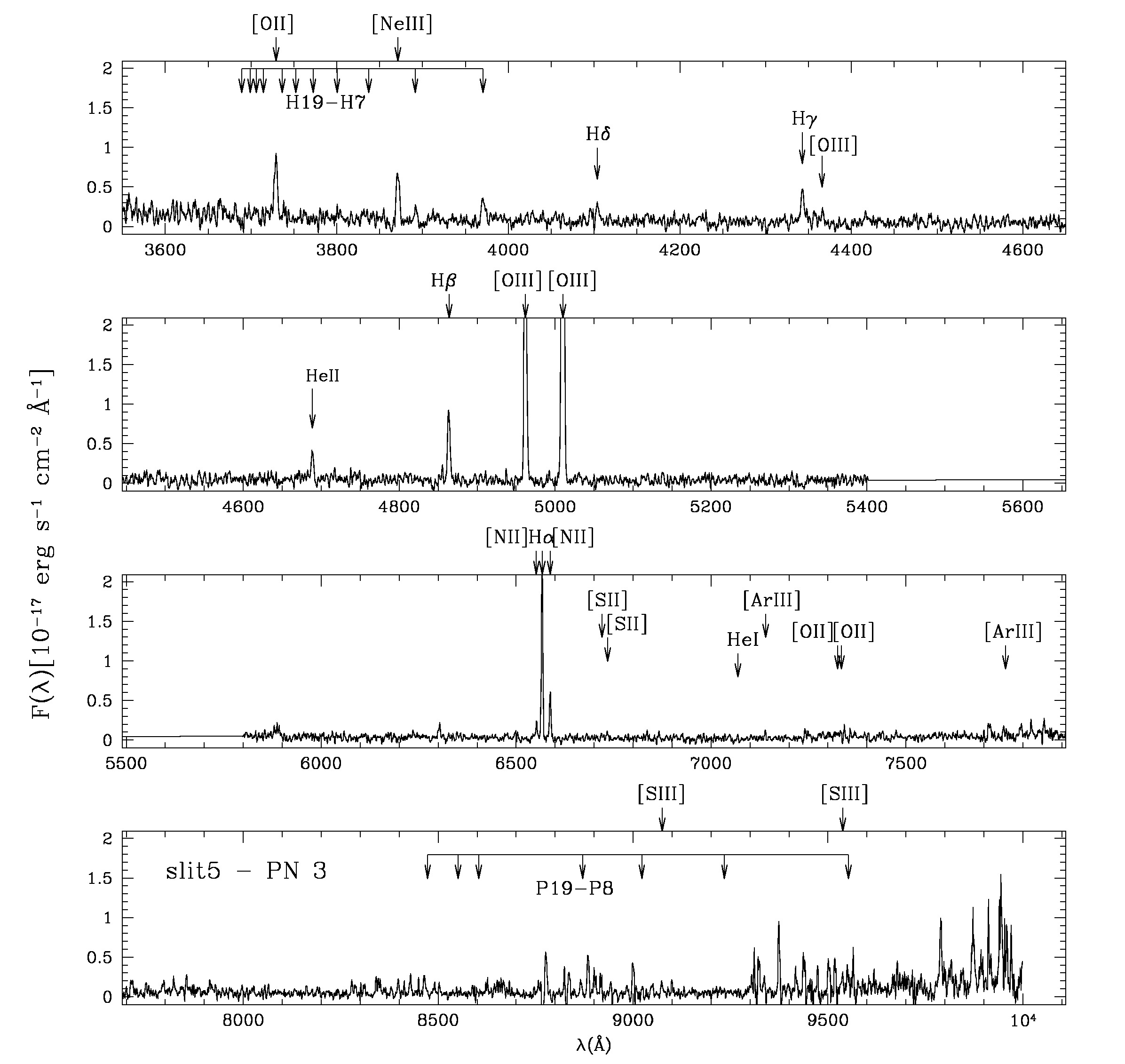
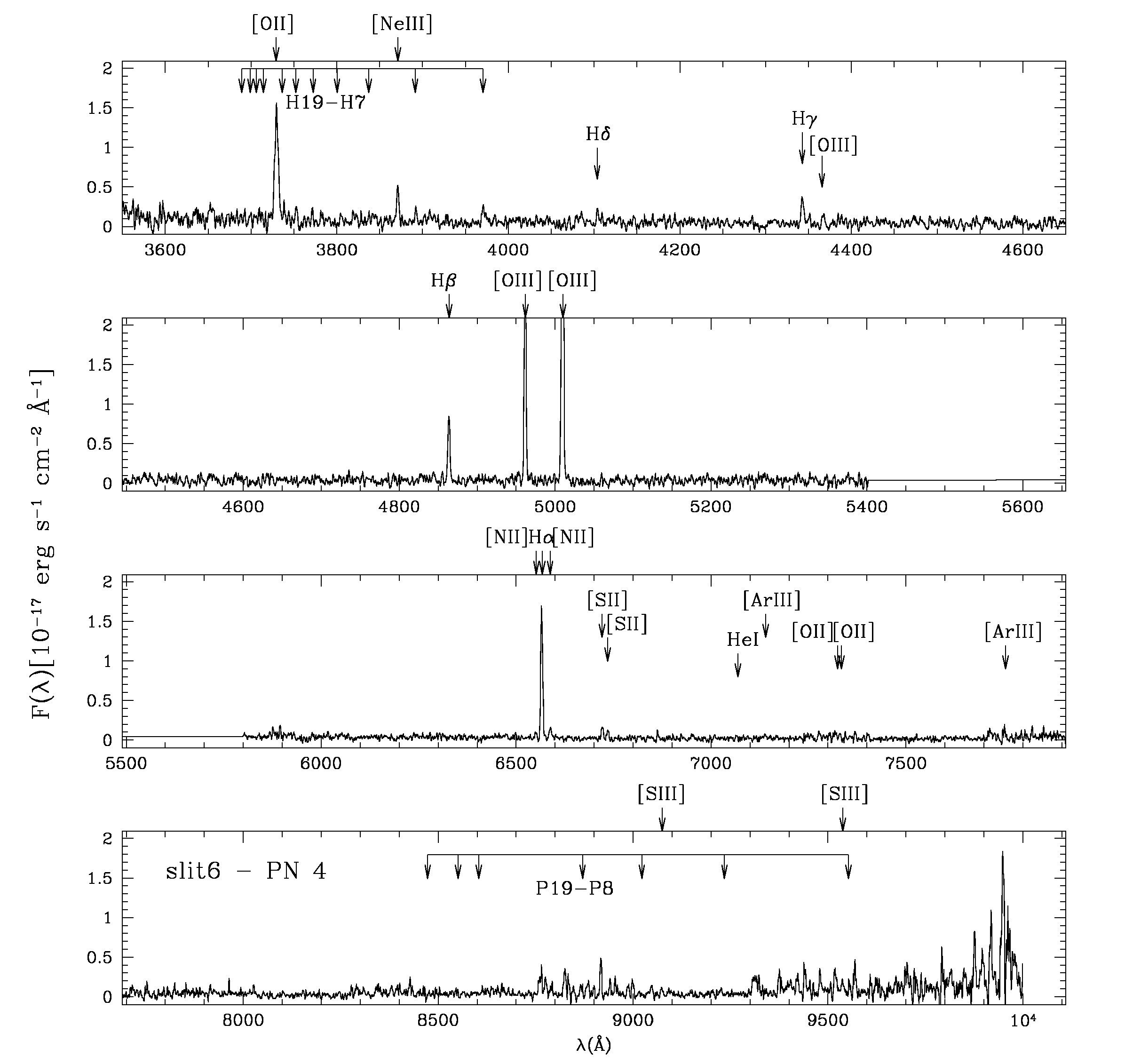
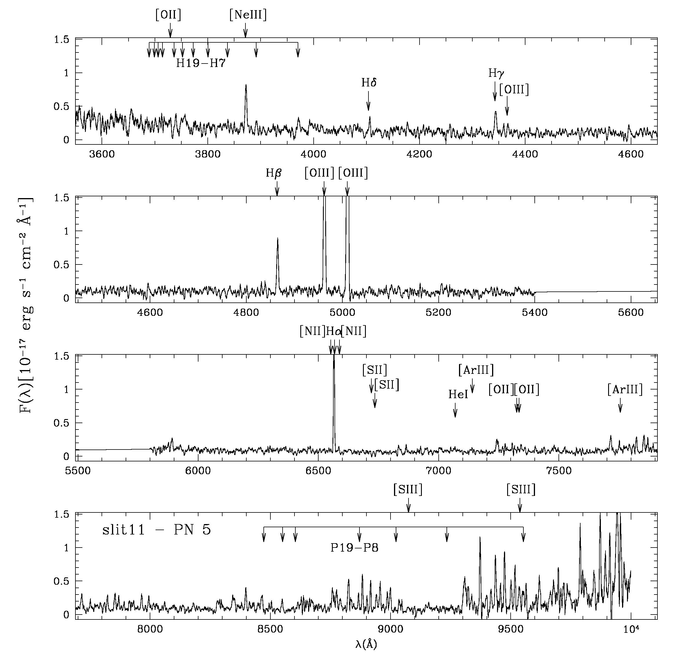
Figure 21 -
LBT/MODS spectra in the blue and red channels for PN-2 in NGC 4449 with indicated all the identified
emission lines. A ~1 Å boxcar filter smoothing was applied to the spectrum to better highlight
the low singal-to-noise features. The spectra have been scaled such that the details are evident.
|
|
Figure 22 -
Same as Fig. 21 but for PN-3.
|
|
Figure 23 -
Same as Fig. 21 but for PN-4.
|
|
Figure 24 -
Same as Fig. 21 but for PN-5.
|
|
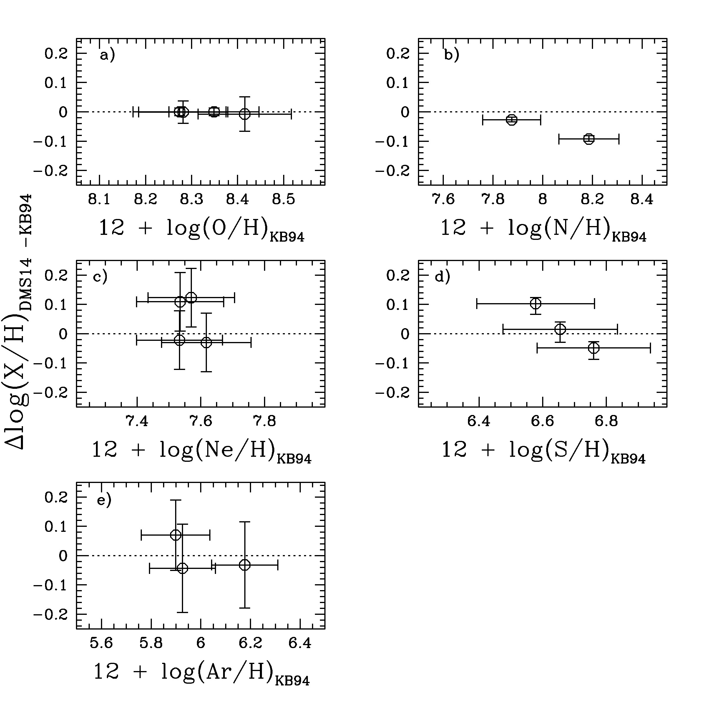
Figure 25 -
Abundance difference due to the use of the new ICFs by DMS14 compared to the old ICFs by KB94, used
in Section 4.2 of this paper (see Appendix for details).
|
Back to article listing |
|
Shortcut to Space Stuff |
| AB/Aug 2017 |
|
|