Back to article listing

Back to article listing |
|
Shortcut to Space Stuff |
| Annibali, F., Morandi, E., Watkins, L.L., Tosi, M., Aloisi, A., Buzzoni, A., Cusano, F., Fumana, M., Marchetti, A., Mignoli, M., Mucciarelli, A., Romano, D., van der Marel, R.P.: |
| "LBT/MODS spectroscopy of globular clusters in the irregular galaxy NGC 4449", 2018, MNRAS, 476, 1942 |
|
|
Summary:
We present intermediate-resolution (R~1000) spectra in the ~3500-10000 Å range of 14 globular
clusters in the magellanic irregular galaxy NGC 4449 acquired with the Multi Object Double Spectrograph
on the Large Binocular Telescope. We derived Lick indices in the optical and the CaII-triplet index in the
near-infrared in order to infer the clusters' stellar population properties. The inferred cluster ages are
typically older than ~9 Gyr, although ages are derived with large uncertainties. The clusters exhibit
intermediate metallicities, in the range −1.2≤[Fe/H]≤−0.7 dex, and typically sub-solar
[α/Fe] ratios, with a peak at ~−0.4 dex. These properties suggest that i) during the first few
Gyrs NGC 4449 formed stars slowly and inefficiently, with galactic winds having possibly contributed
to the expulsion of the α-elements, and ii) globular clusters in NGC 4449 formed relatively
"late", from a medium already enriched in the products of type Ia supernovae. The majority of clusters
appear also under-abundant in CN compared to Milky Way halo globular clusters, perhaps because of the lack
of a conspicuous N-enriched, second-generation of stars like that observed in Galactic globular clusters.
Using the cluster velocities, we infer the dynamical mass of NGC 4449 inside 2.88 kpc to be
M(<2.88 kpc)=3.15 109 MSun.
We also report the serendipitous discovery of a planetary nebula within one of the targeted clusters,
a rather rare event.
|
| Pick up the paper at Astro-ph/1802.02338 | Local link to the PDF version (1.7 Mb) | ||
|
Enhanced HTML/PDF version at the MNRAS site (*) (*) Soon available. May require access password |
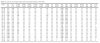 |
Table A1 - Lick and CaII triplet indices derived for globular clusters in NGC 4449 (click for the ASCII file)
|
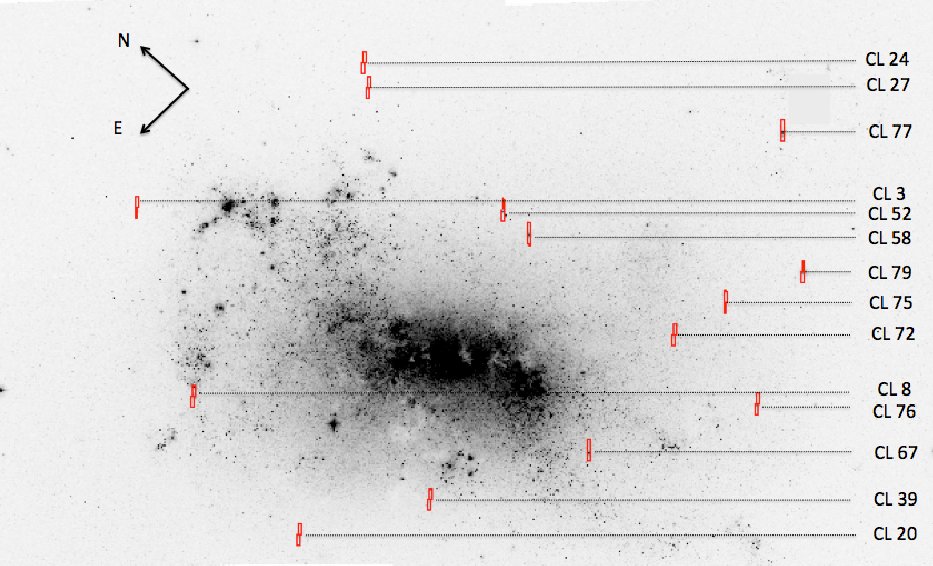 |
Figure 1 -
HST/ACS mosaic image of NGC 4449 in F555W (~V) with superimposed the LBT/MODS 1"x8" slits centered on
star clusters. The cluster identification numbers correspond to those in Annibali et al. (2011b).
|
|
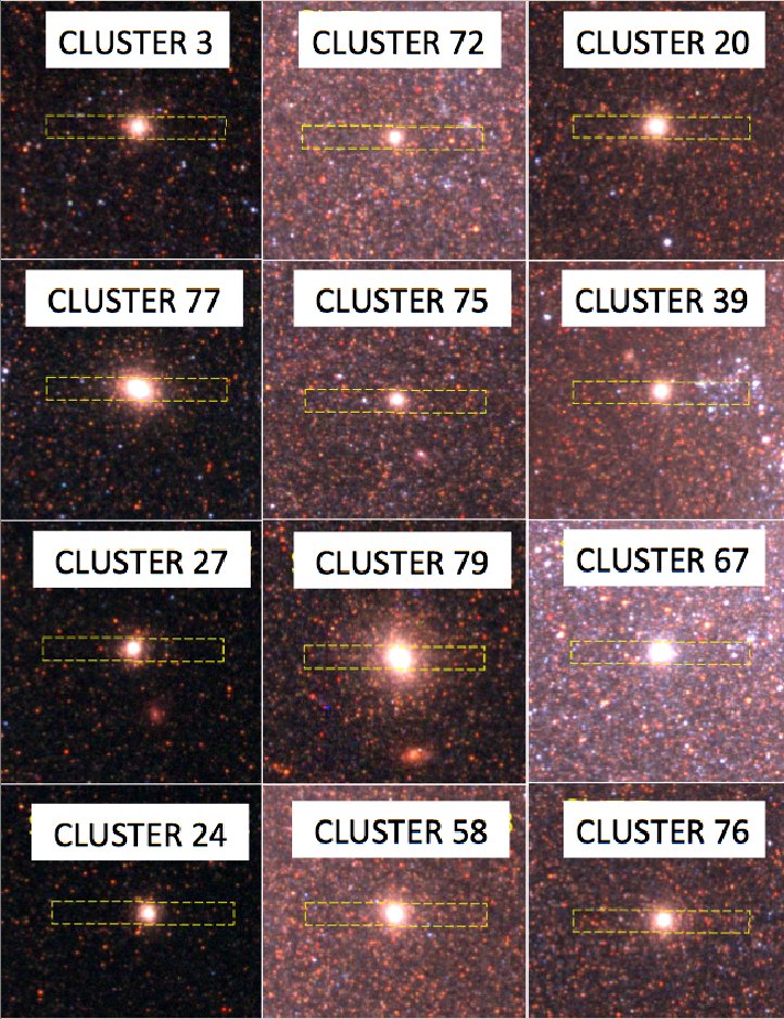
Figure 2 -
HST/ACS color-combined images (F435W=blue, F555W=green, F814W=red) of clusters in NGC 4449 targeted
for spectroscopy with LBT/MODS. In each box, the cluster identification number is that of Annibali et al. (2011b).
Each field of view is 12"x12", and the slit is 1"x8".
|
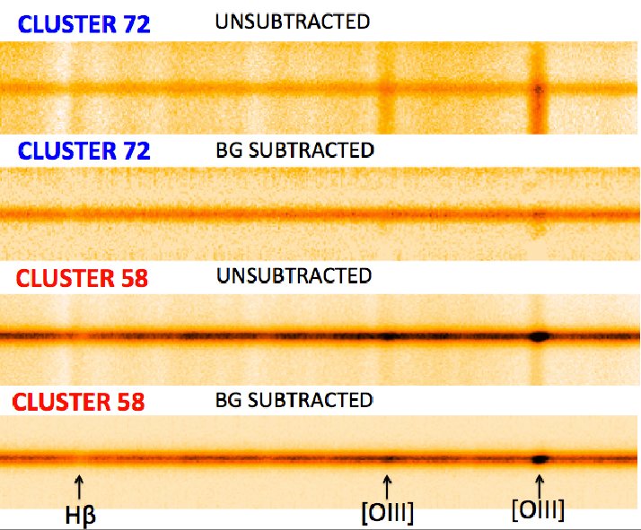 |
Figure 3 -
Two examples of cluster spectra contaminated by emission lines. Portions of the spectra around the Hβ and
[O III]λλ4959,5007 Å lines are shown. For each cluster, the total-combined
un-subtracted spectrum is in the higher row, while the background-subtracted spectrum is just below. Cluster
CL 72 suffers contamination from the diffuse ionized gas in NGC 4449, and some residual emission
is still present after background subtraction. In cluster CL 58, the (modest) contamination from the
diffuse ionized gas in NGC 4449 is optimally removed with the background subtraction; on the other hand,
the cluster exhibits a quite strong centrally concentrated emission.
|
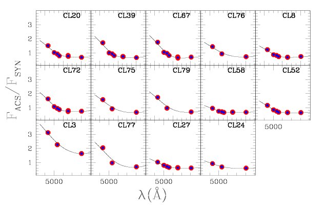 |
Figure 4 -
Effect of differential atmospheric refraction on our cluster spectroscopy. In ordinate, FACS/FSYN
is the ratio between the measured ACS fluxes (in F435W, F555W, F814W, F502N, F550M, F658N, and F660N) and
the Synphot synthetic fluxes (see Section 2 for details).
The curve is the fit obtained adopting a radial basis function (RBF).
|
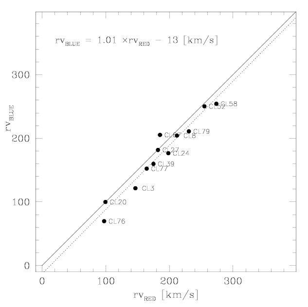 |
Figure 5 -
Comparison between cluster radial velocities obtained with the blue and with the red MODS spectra, respectively.
The solid line is the one-to-one relation, while the dotted line is the linear fit to the data points. Notice
that the displayed velocities have not been corrected here for the motion of the Sun.
|
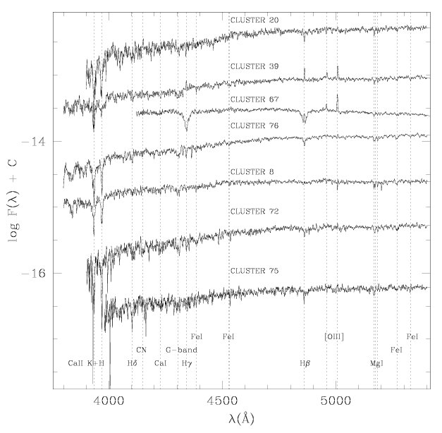 |
Figure 6 -
LBT/ MODS blue calibrated spectra in the rest-frame for clusters CL 20, CL 39, CL 67, CL 76,
CL 8, CL 72 and CL 75 in NGC 4449. Indicated are the most prominent absorption and emission lines.
|
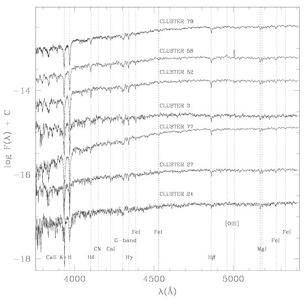 |
Figure 7 -
Same as in Fig. 6 but for clusters CL 79, CL 58, CL 52, CL 3, CL 77, CL 27
and CL 24.
|
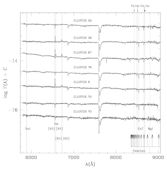 |
Figure 8 -
LBT/MODS red calibrated spectra in the rest-frame for clusters CL 20, CL 39, CL 67, CL 76,
CL 8, CL 72 and CL 75 in NGC 4449. Indicated are the most prominent absorption and emission
lines.
|
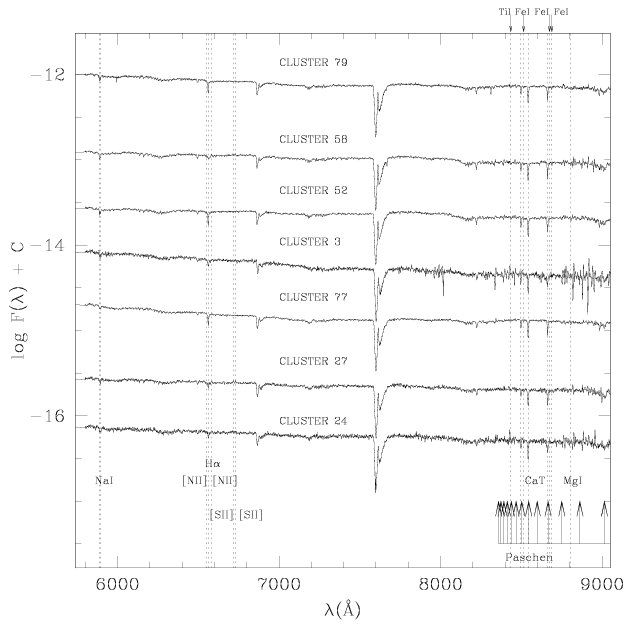 |
Figure 9 -
Same as in Fig. 8 but for clusters CL 79, CL 58, CL 52, CL 3, CL 77,
CL 27 and CL 24.
|
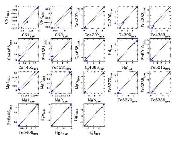 |
Figure 10 -
Comparison between the nominal Lick index values and our measurements for the three Lick standard stars
(HD 74377, HD 84937, and HD 108177) observed during our run.
The solid line is the one-to-one relation, while the dotted line is the least-squares linear fit.
|
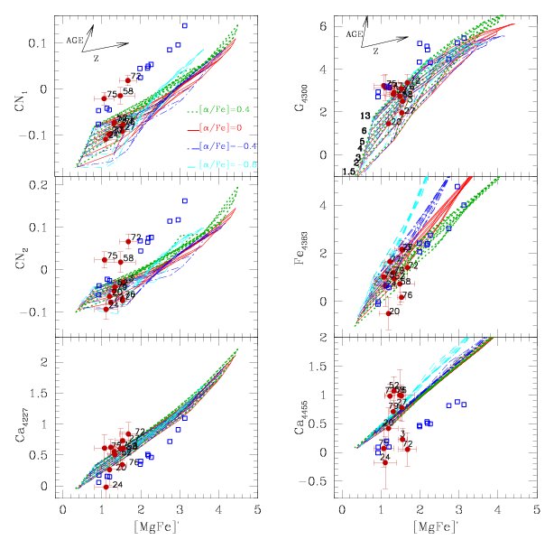 |
Figure 11 -
Comparison of cluster Lick indices (CN1, CN2, Ca 4227, G 4300, Fe 4383,
Ca 4455 versus [MgFe]') with our simple stellar population models. The solid red points are the NGC 4449
clusters from this work, while the open blue squares are the MW halo and bulge globular clusters from
Puzia et al. (2002). The displayed models are for metallicities Z=0.0004, 0.004, 0.008, 0.02, 0.005, ages
from 1 to 13 Gyr, and [α/Fe] = −0.8, −0.4, 0.0, and +0.4.
|
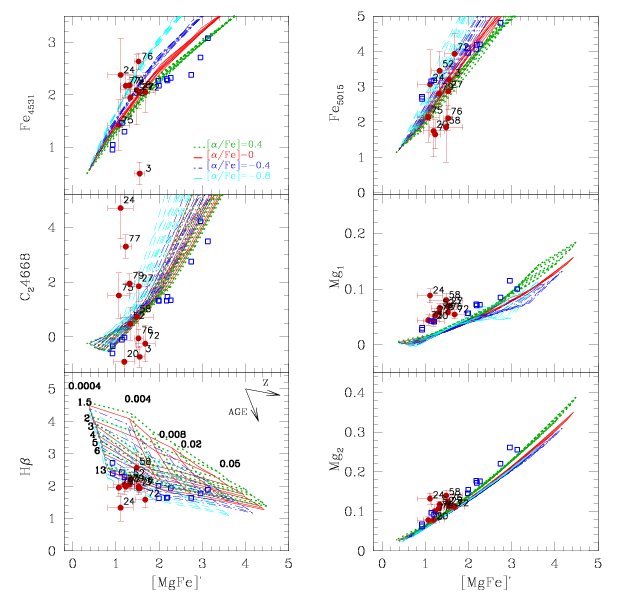 |
Figure 12 -
Same as in Fig. 11 but for the Lick indices Fe 4351, C24668, Hβ, Fe 5015,
Mg1, and Mg2. The metallicity and age labels (Z and Gyr, respectively) refer to the
[α/Fe]=0 models.
|
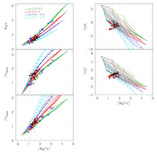 |
Figure 13 -
Same as in Fig. 11 but for the Lick indices Mgb, Fe 5270, Fe 5335, HγA, and HγF.
|
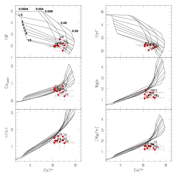 |
Figure 14 -
Cluster Lick indices versus the near infrared CaT* index. The data are for the NGC 4449 clusters, while the
models are our "standard" simple stellar populations for Z=0.0004, 0.004, 0.008, 0.02, 0.005, and ages from 1
to 13 Gyr. Notice that the "standard" models are calibrated on Galactic stars and thus reflect the MW
chemical composition ratios.
|
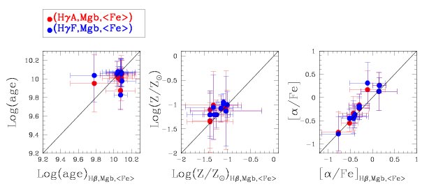 |
Figure 15 -
Ages, metallicities, and [α/Fe] ratios derived for clusters CL 20, CL 76, CL 72, CL 75,
CL 79, CL 58, CL 52, CL 3, CL 77, CL 27 and CL 24 in NGC 4449 using
different combinations of index triplets. The stellar population parameters obtained with the (Hβ, Mgb,
<Fe>) triplet are on the x axes, while the results from the other triplets, as indicated in the legend,
are on the y axes. The solid line is the one-to-one relation. Ages are in units of log10(age [yr]).
The adopted solar metallicity is ZSun=0.018.
|
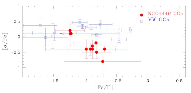 |
Figure 16 -
Distribution of clusters in NGC 4449 and in the MW in the [α/Fe] versus [Fe/H] plane. The displayed
MW clusters belong to the sample of Puzia et al. (2002) and are both halo and bulge globular clusters.
The stellar population parameters of Galactic clusters have been obtained by reprocessing the Lick indices
provided by Puzia et al. (2002) through our models for a self-consistent comparison with the NGC 4449
results.
|
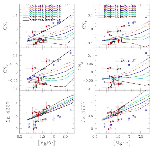 |
Figure 17 -
Distribution of NGC 4449's and MW clusters from Puzia et al. (2002) (full red points and open blue squares,
respectively) in the CN1, CN2, and Ca 4227 vs. [MgFe]' planes. Overplotted are 11 Gyr
old models for different combinations of [α/Fe] and [N/α].
|
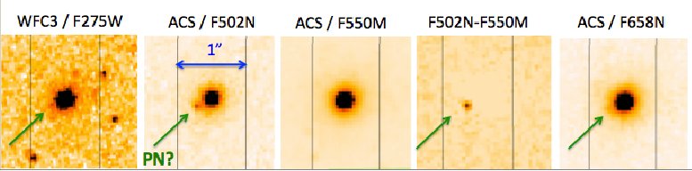 |
Figure 18 -
HST images of cluster CL 58 in different bands: F275W (NUV) from GO program 13364 (PI Calzetti), and
F502N ([O III]), F550M, and F658N (Hα) from GO program 10522 (PI Calzetti). The continuum-subtracted
[OIII] image (F502N−F550M) well shows the presence of a PN candidate in cluster CL 58.
The PN is also detected in the NUV and (with a low signal-to-noise) in Hα. Superimposed on the cluster is
the 1"-wide slit used in our MODS observation.
|
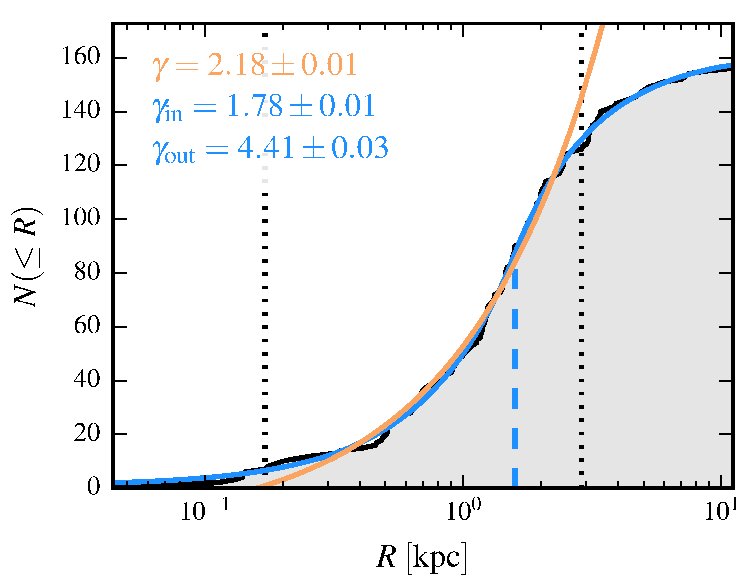 |
Figure 19 -
The cumulative number density profile of globular clusters in NGC 4449. The black line shows the profile
measured from the combined catalogues of Annibali et al. (2011b) and Strader et al. (2012). The orange line
shows the best-fitting profile to the region of interest (marked by vertical dotted lines) assuming that
the underlying density profile is a power-law. The index of the power-law γ is given in orange the
top-left corner. The blue line shows the best-fitting profile to the whole sample assuming that the underlying
density profile is a double power-law with an inner index of γin and an outer index
γout (shown in blue in the top-left corner). The radius at which the power-law index
changes from inner to outer is marked by the blue vertical dashed line. We use the single fit as the best
estimate of the power-law in this region and use the indices from the double fit to provide uncertainties.
|
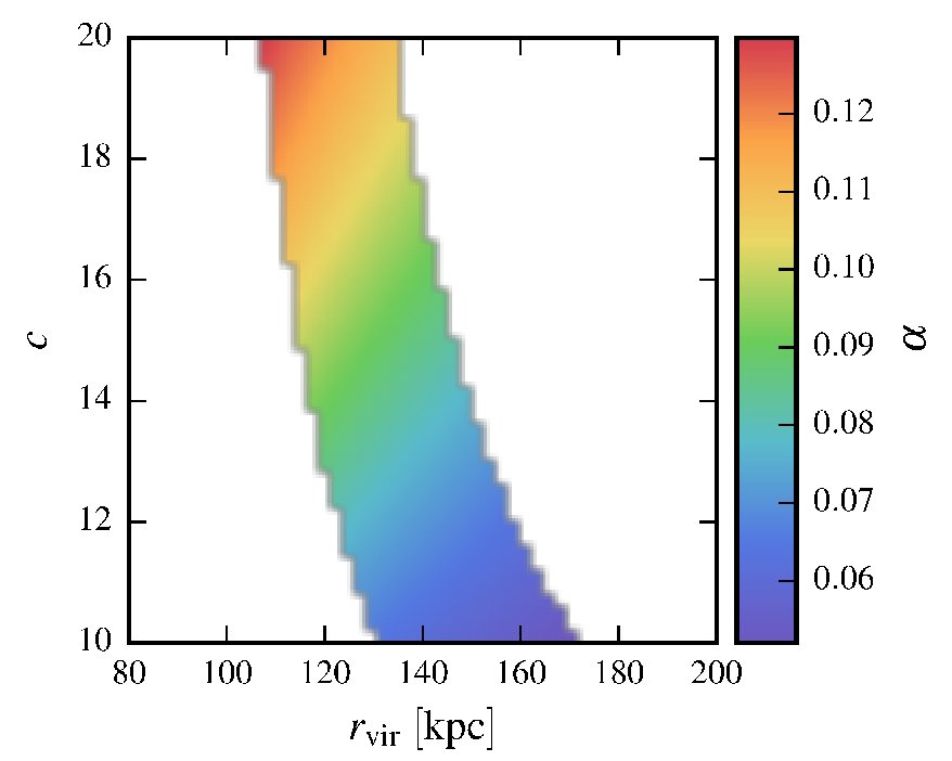 |
Figure 20 -
The variation in potential slope α for a grid of DM halos assumed to be NFW in shape and defined
by a concentration c and a virial radius rvir. To each halo, we fit a power-law over the range
of interest for our mass estimation -- the colour bar shows how the index α of the best-fitting
power-law changes from halo-to-halo. We only show halos with circular velocities at 15.7 kpc of
84±10 km/s to force consistency with HI observations. The white regions are halos with
circular velocities outside of this range.
|
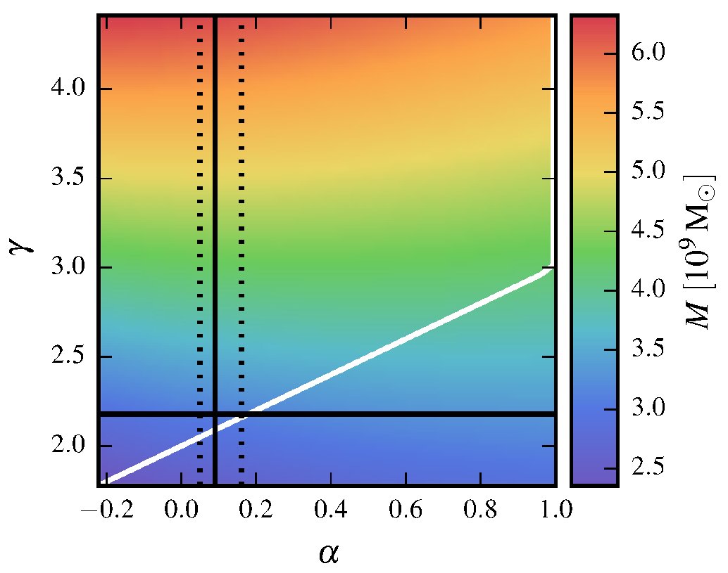 |
Figure 21 -
The variation in estimated mass inside 2.88 kpc as a function of potential slope α and density
slope γ. The range of γ was set by fitting to existing globular cluster data. The range of
α was set by assuming that mass follows light, in which case α = min(1, γ−2)
(marked by the white line), as this range was larger than that estimated from considering DM halo models
(highlighted by vertical dotted lines). The solid black lines show our best estimates for α and γ,
and their intersection shows the adopted best mass estimate. The minimum and maximum masses in this grid
set our uncertainties.
|
Back to article listing |
|
Shortcut to Space Stuff |
| AB/Mar 2018 |
|
|