Back to article listing

Back to article listing |
|
Shortcut to Space Stuff |
| Buzzoni, A., Altavilla, G., Fan, S., Frueh, C., Foppiani, I., Micheli, M., Nomen, J., Sànchez-Ortiz, N.: |
| "Physical characterization of the deep-space debris WT1190F: a testbed for advanced
SSA techniques" 2019, Advances in Space Research, 63, 371 |
|
|
Summary:
We report on extensive BVRcIc photometry and low-resolution (λ/Δλ ~ 250) spectroscopy of the deep-space debris
WT1190F, which impacted Earth offshore from Sri Lanka, on 2015 November 13. In spite of its likely artificial origin
(as a relic of some past lunar mission), the case offered important points of discussion for its suggestive connection with
the envisaged scenario for a (potentially far more dangerous) natural impactor, like an asteroid or a comet.
Our observations indicate for WT1190F an absolute magnitude Rc = 32.45±0.31, with a flat dependence of reflectance
on the phase angle, such as dRc/df ~ 0.007±2 mag deg-1. The detected short-timescale variability suggests that the
body was likely spinning with a period twice the nominal figure of Pflash = 1.4547±0.0005 s, as from the observed lightcurve.
In the BV RcIc color domain, WT1190F closely resembled the Planck deep-space probe. This match, together with a
depressed reflectance around 4000 and 8500 Å may be suggestive of a grey (aluminized) surface texture.
The spinning pattern remained in place also along the object fiery entry in the atmosphere, a feature that may have
partly shielded the body along its fireball phase perhaps leading a large fraction of its mass to survive intact, now lying
underwater along a tight (~1x80 km) strip of sea, at a depth of 1500 meters or less.
Under the assumption of Lambertian scatter, an inferred size of 216±30/√ (α/0.1) cm is obtained for WT1190F.
By accounting for non-gravitational dynamical perturbations, the Area-to-Mass ratio of the body was in the range
(0.006 ≤ AMR ≤ 0.011) m2 kg−1.
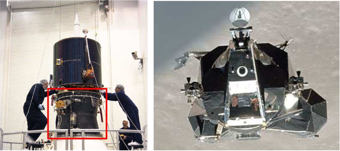
Both these figures resulted compatible with the two prevailing candidates to WT1190Fs identity, namely the Athena
II Trans-Lunar Injection Stage of the Lunar Prospector mission, and the ascent stage of the Apollo 10 lunar module,
callsign Snoopy. Both candidates have been analyzed in some detail here through accurate 3D CAD design mockup
modelling and BRDF reflectance rendering to derive the inherent photometric properties to be compared with the
observations.
|
| Pick up the paper at Astro-ph/
(Soon available) |
Local link to the PDF version (1.7 Mb)
(For personal use only) |
||
|
Enhanced HTML/PDF version at the AdSR site (*) (*) May require access password |

|
Figure 1 -
A historical timeline of the WT1190F V and R apparent
magnitude, as from the DASO database, back to year 2009. The data
collect observations for the alias objects UW8551D, UDA34A3 and
9U01FF6, later found to be identified with the same body. The full
sample consists of 125 V and 230 R magnitude estimates. To these
data one has to add a further set of 1271 Gunn r magnitudes by the
G45 SST Atom Site Obs in late 2015 (oveplotted in the R panel as
small x markers).
|
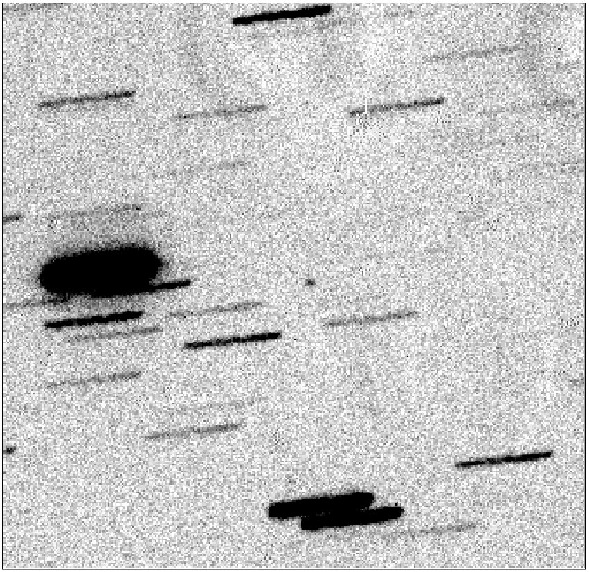
| Figure 2 -
An illustrative frame of WT1190F detection at
01:21:34 UTC (mid-exposure time, see Table 1) of 2015 November
8. The target is imaged in the Johnson-Cousins Rc band with a
420 s exposure time. The cropped field here is 3.1 arcmin across.
At the moment of this exposure, the object was 518 000 km away
from us. Thanks to the on-target telescope tracking, WT1190F is
clearly detected as a point source at the center of the image, with a
magnitude Rc = 20.54.
|
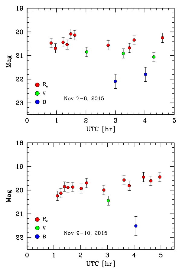 |
Figure 3 -
The WT1190F B, V, R lightcurve along the Loiano observing runs of 2015 November 7-8 and November 9-10. The x-axis
timeline refers to the UTC hours respectively of Nov 8 and Nov 10.
|
|
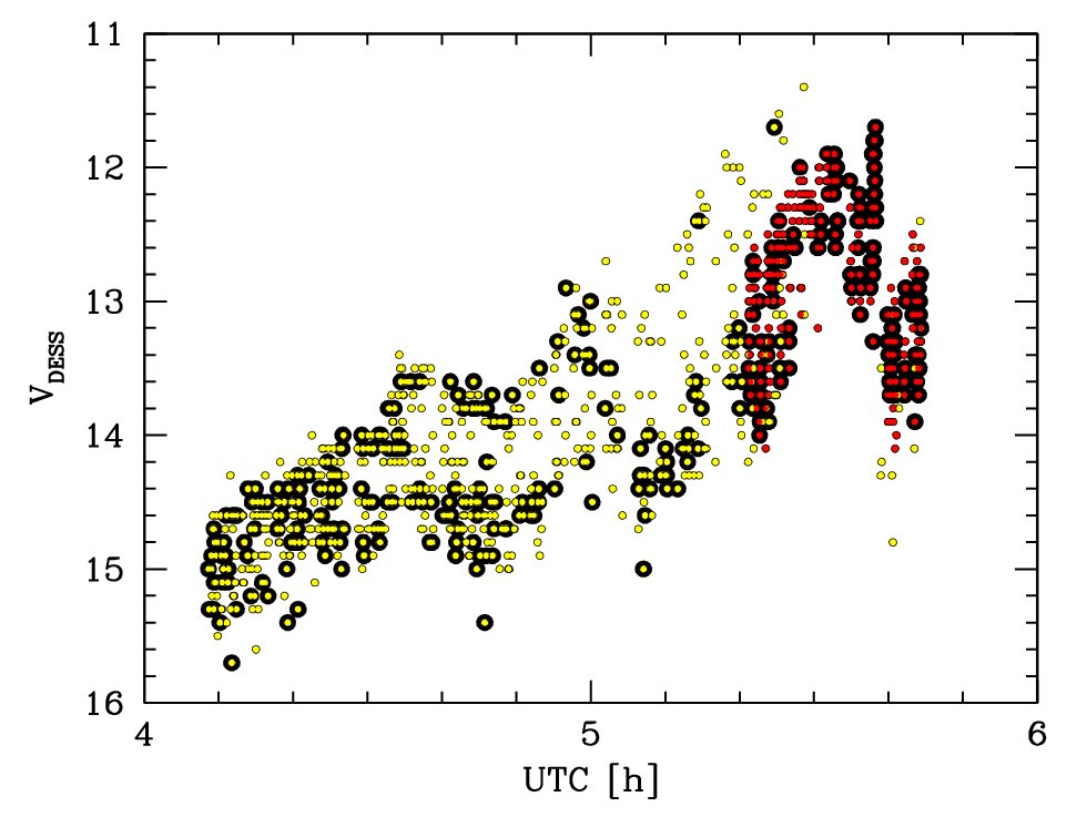
Figure 4 -
The full DeSS data set of 1125 V -band observations along
the WT1190F final approach of 2015 November 12-13. The magnitude sample of the Tracker (yellow markers) and Antsy (red
markers) telescopes (708 and 417 points, respectively) are merged in
the plot, without relative offset correction. Bold points (for the two
telescopes) refer to the astrometric DASO measurements (SànchezOrtiz et al., 2015). The x-axis timeline is in
UTC hours of November 13.
|
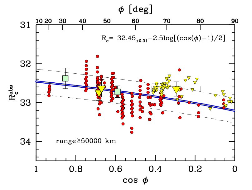 |
Figure 5 -
The WT1190F R absolute magnitude with changing orbital phase angle φ. The relevant DASO dataset of the 190 observations
in year 2015 with geocentric distance in excess of 50 000 km is merged (red dots), after statistical correction,
as explained in the text. These data are complemented by the Loiano observations of 2015 November (the three big triangle
markers, as an average of each observing night), together with the individual measures of the November 12-13 approaching
sequence (small yellow triangles). The G45 (SST Atom Site Obs.) Gunn r magnitude series are also joined, as an average
for each observing night (big square markers) after correction to the Johnson-Cousins R band, as discussed in the text.
The fitting curve, by assuming luminosity to be proportional to the target illuminated area, leads to an absolute
magnitude of Rcabs = 32.45±0.31, as labeled in the plot.
|
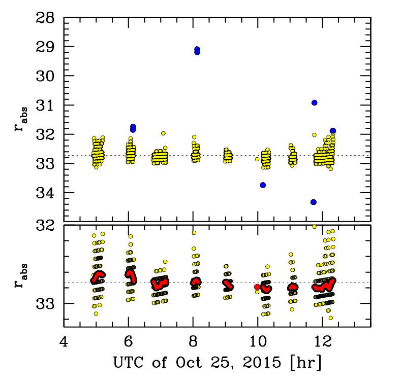 |
Figure 6 -
The 1004 Gunn r observations of 2015 October 25 by the
G45 SST telescope at the Atom Site Obs. (USA) are displayed, after
correcting for distance to an absolute magnitude scale. Interloping
the quiescent underlying behaviour of WT1190F (yellow dots), one
can recognize in the upper panel a remarkable series of flares and
dimming events (blue dots), on timescales of seconds, exceeding a
3s random fluctuation around the average magnitude of the data.
Besides this abrupt and striking variation, the G45 data do not show
any sign of coherent trend on slower timescales, as shown by the
smoothing running average (red dots) displayed in the zoomed in
point distribution of the lower panel.
|
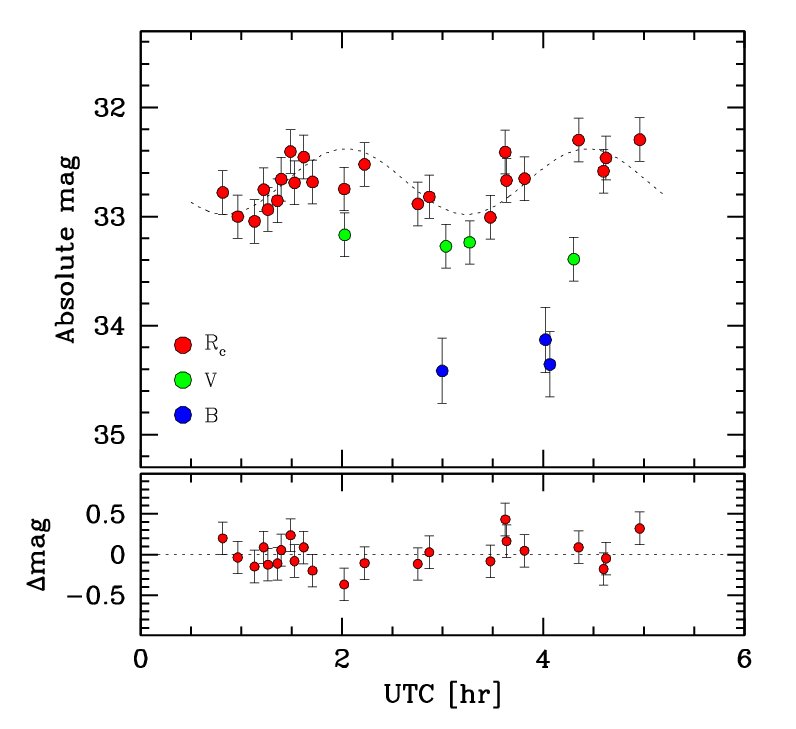 |
Figure 7 -
The Loiano observations of Fig. 3 are merged in the upper
plot, after rescaling to absolute magnitudes. The displayed pattern
in both 2015 November nights for the WT1190F R magnitude to
change on a tentative timescale of 2.4 hours is reinforced here, as a
(somewhat speculative) evidence of a coherent object variability with
an amplitude of about 0.7 mag (dotted curve). The magnitude residuals with
respect to a fitting sinusoidal curve have a σR = 0.18 mag
(rms) and are displayed in the lower panel. See text for a discussion.
|
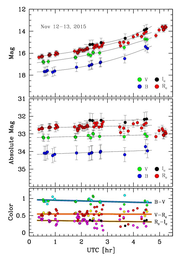 |
Figure 8 -
The B, V, Rc, Ic photometry of WT1190F during its final Earth approach of 2015
November 12-13, as seen from Loiano,
are reported in the upper panel. Once rescaling for the (quickly reducing) distance,
the inferred absolute magnitudes and colors are
shown, along the same night, in the mid and lower panels of the
figure, respectively. The fit of these data is reported in the set of
eq. (5) relations. Note the abrupt drop in objects R-band absolute
luminosity about 05:00 UTC (as in mid panel). The x-axis timeline
in the figure is in UTC hours of Nov 13.
|
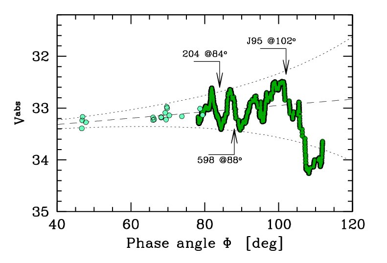 |
Figure 9 -
The absolute V-band magnitude trend with orbital phase
angle f along the final approaching trajectory of WT1190F. The Nov
12-13 DeSS observations (green solid curve), for φ > 78o are merged
with the Loiano coarser set of measures, sampling lower phase-angle
figures. Note the diverging oscillating regime of WT1190F luminosity on
~20 min timescales, that abruptly sets in place with φ
approaching and exceeding a square-angle illumination aspect. To
better single out the trend, DeSS data have been smoothed with a 30-
point running average. As discussed in the text, in their comparison
with the Loiano dataset, both Tracker and Antsy magnitudes have
been corrected accordingly. The relevant timing of Campo dei Fiori
(code 204), Loiano (598) and Great Shefford (J95) lightcurve
sampling of Fig. 11 is marked on the plot.
|
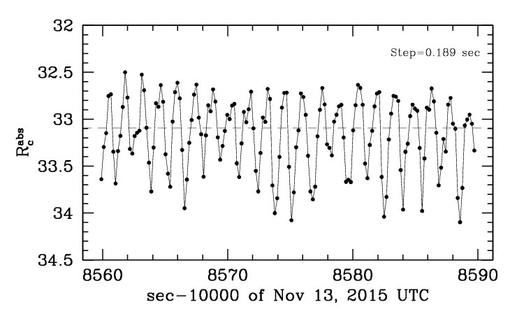 |
Figure 10 -
The quick variability of WT1190F clearly appears in
this R-band trailing frame from Loiano, taken at 05:09:34 UTC of
2015 November 13 (see Table 2). A total of 21 pulses can easily
be recognized in the figure, suggestive of a flashing period slightly
shorter than 1.5 s. The time span of target trail across the CCD
pixels, for this frame, is 0.189 s px-1.
|
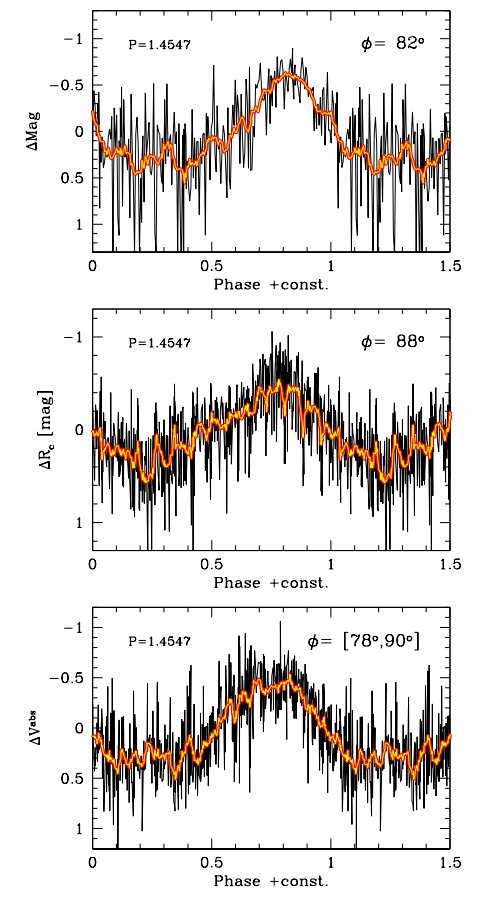 |
Figure 11 -
The WT1190F lightcurve by phasing observations with
the short flashing period of eq. (8). The three different datasets
of Buzzi & Colombo (2015, Campo dei Fiori Obs.; upper panel),
Loiano (mid panel) and DeSS (Tracker telescope; lower panel) are
displayed, for comparison. For a better reading, the raw data distribution
is smoothed with a 15-point running average (thick solid line).
The geometrical circumstance of the orbital phase angle f spanned
by the observations is reported top right in each panel.
|
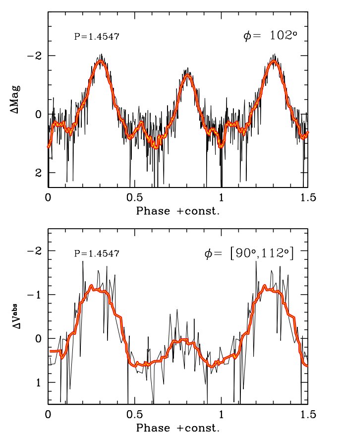 |
Figure 12 -
Same as Fig. 11, but for two datasets taken at orbital
phase angles larger than 90o, namely the Birtwhistle (2015) data
taken at Great Shefford Obs. (upper panel) and the DeSS data
(Tracker telescope; lower panel). Compared to the previous figure, a substantial
change in the lightcurve shape is evident, with
an intervening secondary maximum that keeps growing midway of
the curve. This transient feature (that only appeared in the very
last minutes before the atmosphere entry of WT1190F) is striking in
the Great Shefford data and found full confirmation from the DeSS
observations.
|
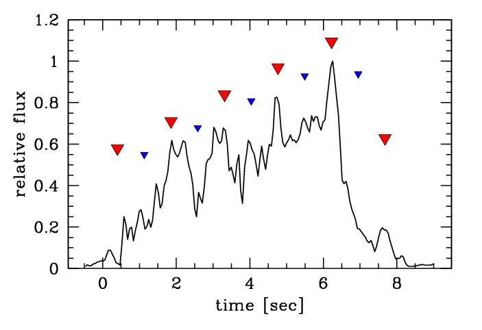 |
Figure 13 -
The apparent luminosity of WT1190F during its atmosphere burning phase,
according to the Jenniskens et al. (2016)
observations. At the timeline origin of the plot, the object started to
brighten at a height of 73 km reaching a maximum peak luminosity
6.3 s later, about 50.5±2.5 km. Notice the flashing behaviour along
the atmosphere entry, which seems to be consistent with eq. (8) (primary
and secondary peaks, as from Fig. 12, are sketched respectively
by red and blue triangles along the curve).
|
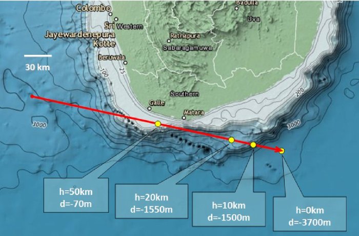 |
Figure 14 -
The WT1190F entry trajectory superposed to the bathimetric map of Sri Lanka
offshore, according to National Centers of
Environmental Information of the NOAA (USA). Labelled on the plot are the
ballistic reference altitude (in kilometers) and the underlying
sea depth (in meters) at some reference points along the trajectory.
See text for full discussion.
|
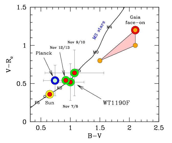 |
Figure 15 -
The (B−V ) versus (V−Rc) average colors of WT1190F
along the three observing runs of 2015 November, from Loiano. The
target colors are compared with other reference objects, namely the
Planck and Gaia spacecraft, the Sun, and the locus of Main Sequence
stars, according to the Pecaut & Mamajek (2013) calibration (solid
curve, labeled with the stellar spectral type). WT1190F appears to
be slightly redder than the Sun, but very close in color to Planck.
It would also quite well match the colors of a star of spectral type K3.
|
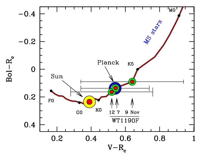 |
Figure 16 -
The reference framework of Fig. 15 is replied here
to assess the bolometric correction to the Rc band. The average
(V−Rc) color of WT1190F along the three observing nights of
2015 November intercepts the Pecaut & Mamajek (2013) stellar calibration
to derive a confident estimate of the bolometric correction
about (Bol−Rc) ~ 0.13±0.05 mag. Note, again, the close match of
WT1190F with the the Planck deep-space probe.
|
 |
Figure 17 -
The WT1190F location in the (Rc−IRc) versus (B−RRc)
color domain, according to the Loiano observations of 2015 November 12-13. Compared with
the Pecaut & Mamajek (2013) stellar locus, the object appears now with an
exceedingly blue (Rc−Ic)
color, suggestive of a reduced reflectance in the Ic band. To further
investigate this feature, we also report in the plot the expected
colors for different materials extensively used in spacecraft and rocket
assembly, as from the Cowardin (2010a) and Cowardin et al. (2010b)
lab measurements. The point caption is: 1 = GaAs solar panel; 2
= std solar panel; 3 = Impacted MLI (Al+Cu Kapton sandwitched
with beta cloth substitute); 4 = Al Kapton (inner side facing spacecraft);
5 = Al Kapton (outer side facing space); 6 = Mylar; 7 = Al
backing solar cell (facing space); 8 = Cu Kapton (facing space); 9
= Al backing solar cell (facing spacecraft); 10 = Cu Kapton (facing
spacecraft).
|
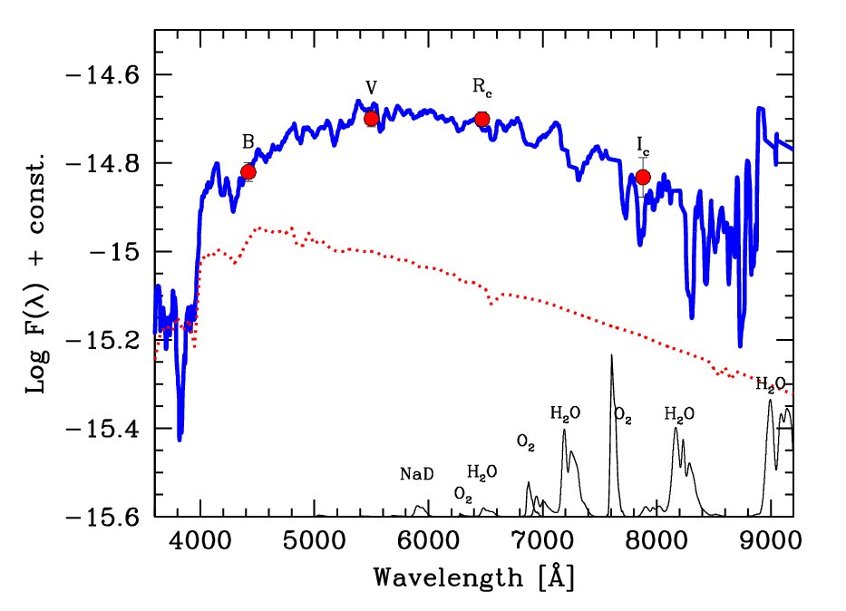 |
Figure 18 -
The WT1190F spectrum, taken from Loiano with the
BFOSC camera, along the night of 2015 November 12-13. Two 300 s
exposures with the grisms GR3 (blue) and GR5 (red) have been
matched, spanning the wavelength region 3500-6000 Å with a 2.7 Å
px-1 dispersion, and 5300-9500 Å with a 4.0 Å px-1 dispersion,
respectively. The spectral resolving power was degraded here to
roughly 100 Å FWHM to improve the S/N ratio still maintaining
the relevant shape of the SED. Correction for O2 and H2O telluric
absorption (according to the pattern sketched in the figure, in arbitrary
units, as labelled) has been carried out as discussed in the
text. A consistent comparison with B, V, Rc, Ic multicolor photometry
(as from Table 3 data) is displayed (big red dots), by converting
the mean magnitudes into monochromatic fluxes, according to Buzzoni (2005).
The solar spectrum is displayed (red dotted line) with
arbitrary offset, for comparison.
|
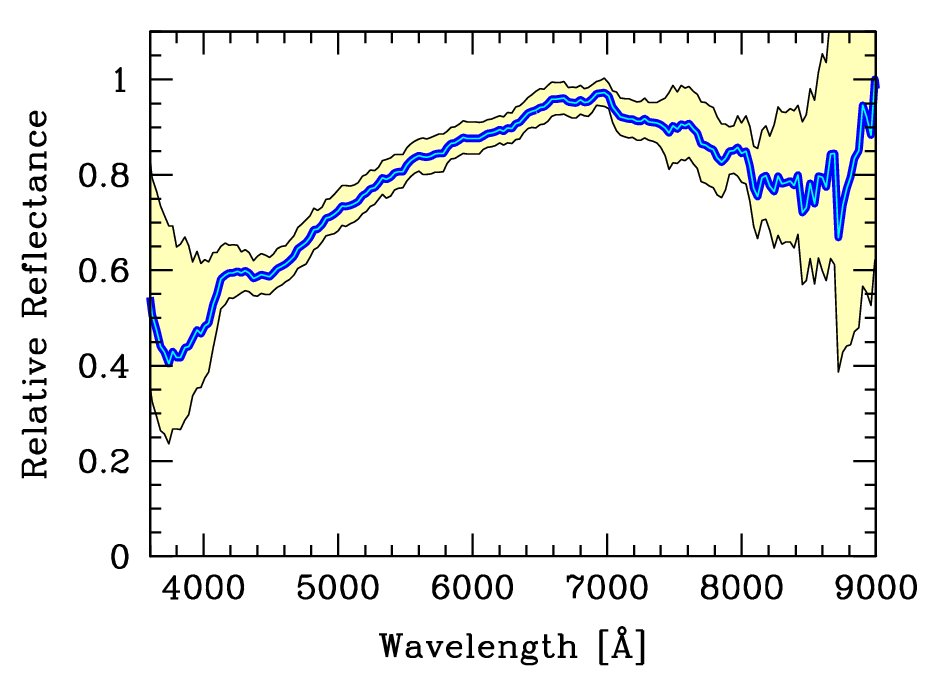 |
Figure 19 -
The WT1190F relative reflectance computed by dividing the observed flux
of Fig. 18 by the synthetic solar spectrum. The
resulting ratio was finally normalized to a unity peak. For its sharply
reduced response about 4000 Å and a shallower dip, about 8500 Å, the
curve may be suggestive of a prevailing presence of Aluminum in the surface texture of the object.
|
|
Figure 20 -
Left panel: the Lunar Prospector spacecraft with its Trans-Lunar
Injection Stage (TLIS) framed within the red box. Picture is
courtesy of NASA and it is publicly available
here .
Right panel: the Lunar Module LM-4 Snoopy of the Apollo 10 mission. The picture was
taken on May 23, 1969, with Snoopy in its course from the Moon to dock again with the
Command Module Charlie Brown. Picture is courtesy of NASA and it is publicly available
here .
|
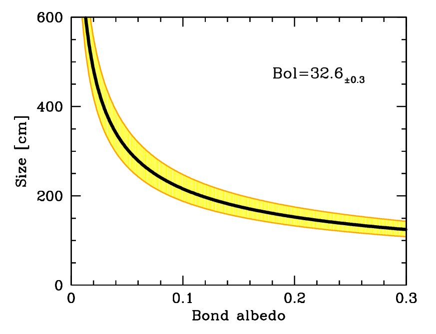 |
Figure 21 -
The expected size versus Bond albedo relationship for
WT1190F, according to eq. (13). A bolometric absolute magnitude
Bol = 32.6±0.3 is assumed for our calculations together with a
Lambertian scattering law for the reflecting body.
|
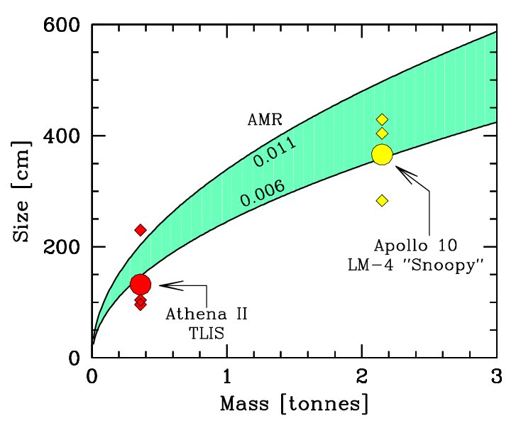 |
Figure 22 -
The expected location of the Apollo 10 LM Snoopy
and the Lunar Prospector TSLI upper stage in the mass versus size
domain, compared with the theoretical locus for the AMR ranging between
0.011 and 0.006 m2 kg-1, as labeled on the plot. For
each object, an effective size is derived (big dots) as the geometric mean
of the corresponding three dimensions (small diamonds in
the plot). This is (2.83 × 4.04 × 4.29)1/3 = 3.66 m for Snoopy and
(1.00 × 1.00 × 2.30)1/3 = = 1.32 m for TLIS. Notice that,
in spite of the large structural difference, both Snoopy and the TSLI module
consistently match the AMR lower envelope, that is for AMR ~ 0.006 m2 kg-1.
|
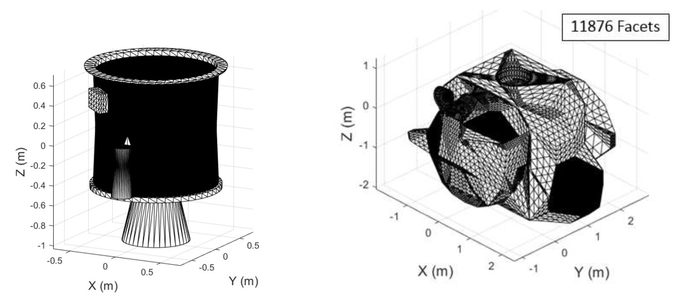 |
Figure 23 -
The rendered TLIS (left panel) and Snoopy (right panel) mesh models. A total of
2902 and 11876 facets have been assumed for the two targets, respectively.
|
 |
Figure 24 -
The absolute magnitude of Snoopy and TLIS mockups,
with varying the phase angle f, according to our synthetic
photometry, is compared with WT1190Fs observations. The latter are from
Fig. 5, once accounting for eq. (12) to convert Rc photometry to
bolometric. If Lambertian reflection is assumed in our BRDF
treatment, at φ = 0, the Snoopy mockup displays an absolute magnitude
of Bolo = 31.36±0.15, while a corresponding value of 33.35±0.06 is
obtained for the TLIS rocket upper stage. Notice for both models
a steeper trend than WT1190Fs absolute luminosity with increasing the orbital phase angle, φ.
Error bars are attached to average magnitudes for each φ configuration as the rms of some
150 individual estimates, by randomly changing mockups orientation in our synthetic photometry.
|
Back to article listing |
|
Shortcut to Space Stuff |
| AB/Dec 2018 |
|
|