Back to article listing

Back to article listing |
|
Shortcut to Space Stuff |
| Buzzoni, A., Guichard, J., Alessi, E.M., Altavilla, G., Figer, A., Carbognani, A. & Tommei, G.: |
| "Spectrophotometric and dynamical properties of the soviet/russian constellation of Molniya satellites" 2020, Journal of Space Safety Engineering, 7, 255 |
|
|
Summary:
We report on the extended observing campaign of the surviving Soviet/Russian spacecraft Molniya,
carried out in the years 201417 at Mexican and Italian telescopes. Spectrophotometry and astrodynamical
analysis have been carried out for all the 43 demised payloads still in uncontrolled HEO orbit at late 2017,
in order to assess dynamical and reflectance properties of such a wide family of virtually identical
orbiting objects, as well as their long-term orbit evolution, according to full historic Two-Line Elements (TLE)
datasets in synergy with mathematical modeling to properly size up the prevailing effect of lunisolar
perturbation and atmospheric drag.
|
|
Enhanced HTML/PDF version at the JSSE site (*) (*) May require access password |
Local link to the PDF version (500 Kb)
(For personal use only) |
||
|
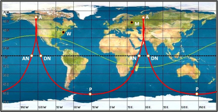
Figure 1 -
An illustrative example of Molniya orbit ground track. Two 12-hr orbits are displayed to span a full day.
The nominal orbital parameters are assumed, for illustrative scope, according to [2]. Note the extremely
asymmetric location of the ascending (AN) and descending (DN) nodes, due to the high eccentricity of the orbit,
and the perigee location (P), always placed in the Southern hemisphere. Along the two daily apogees (A),
the satellite hovers first Russia and then Canada/US. The visibility horizon (i.e. the foot print)
attained from the Russian apogee, is marked by the yellow line. Notice, in this example, that both
Washington (W) and Moscow (M) are in sight from the spacecraft.
|
|
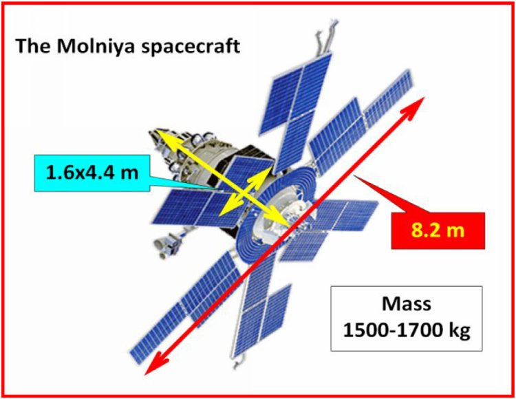
| Figure 2 -
A sketch of a Molniya spacecraft with its characteristic daisy look, as inspired by the six big solar panels.
The spacecraft sports a size of 4.4×8.2×8.2 m, with a typical mass about 15001700 kg. Note that the two high-gain
antennas, symmetrically placed at the two sides of the bus, are not displayed in this figure.
|
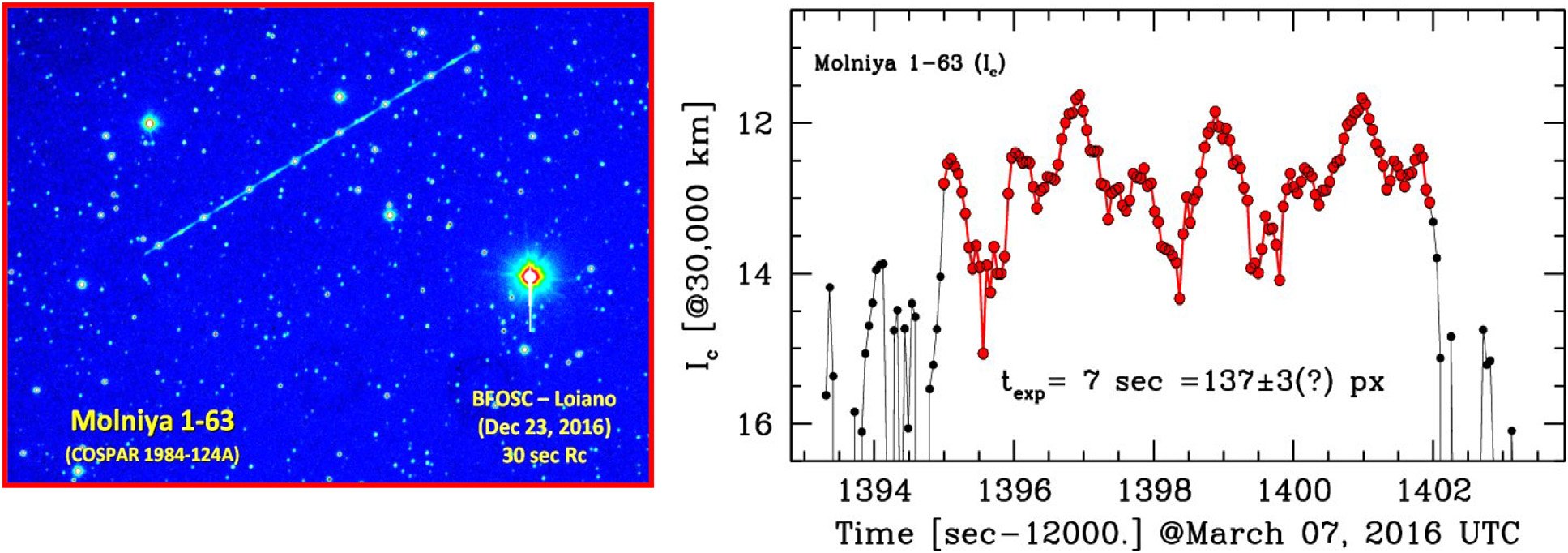 |
Figure 3 -
(Left panel): a 30 sec R-band frame tracking Molniya 1-63 across the sky of Loiano, during a 2016 observing session.
Note the repeated dot-dashed pattern along the satellite trace. (Right panel): the extracted track of Molniya 1-63
from an I-band LFOSC frame taken in Cananea, on 2016 March 7. The 7 sec exposure clearly shows a repeating pattern
over timescales about 4 s. The very short (but finite) time for the CCD shutter to start/stop the exposure makes
the exact gcut hof the track (both in pixel/time and magnitude) somewhat uncertain, as discussed in the text.
The adopted satellite track, taking a total of 137 bona fide "switched-on" pixels, is marked in red for this example.
|
|
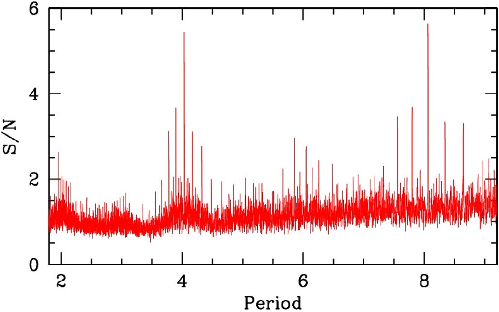
Figure 4 -
A PDM score plot for a set of I-band frames of Molniya 163 (one of which is shown in the right panel of Fig. 3),
in search for the likely periodicity values. Note the period clustering around the value of P~4 s and its
corresponding 1/2x and 2x aliases around P~2 and 8 s, respectively, as discussed in the text. According to
our analysis, the spacecraft appears eventually to spin with a period P = 4.031 s.
|
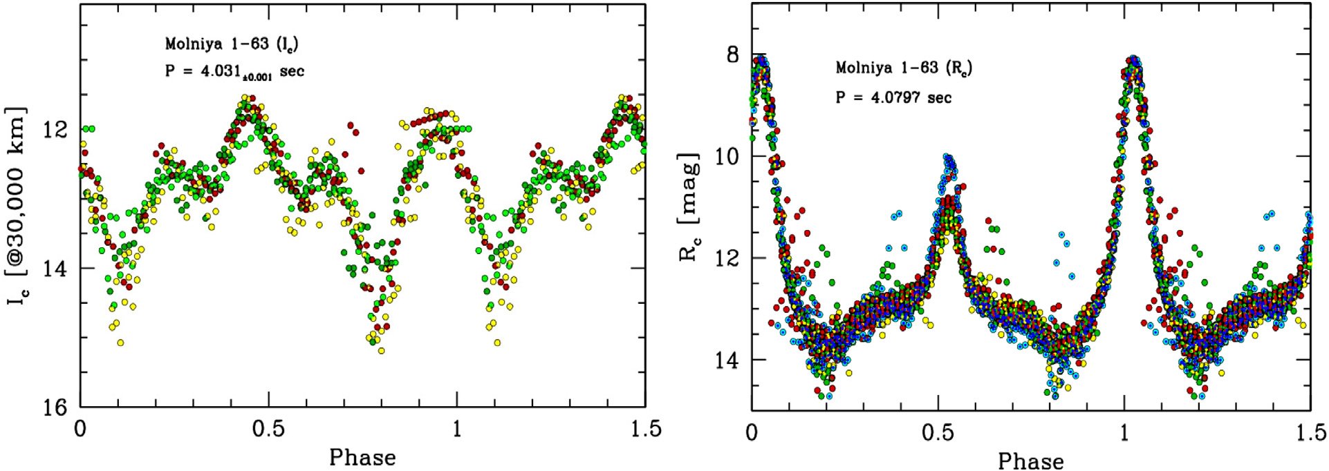 |
Figure 5 -
The folded I- and R-band lightcurve of Molniya 163, as seen from Cananea (left panel) and Loiano (right panel),
along two 2016 observing runs. In both cases (and throughout in this paper) apparent magnitudes are scaled to a
fixed reference distance of 30,000 km. Note the quite different pattern, with the flashing behavior of the Loiano
observations, as discussed in the text.
|
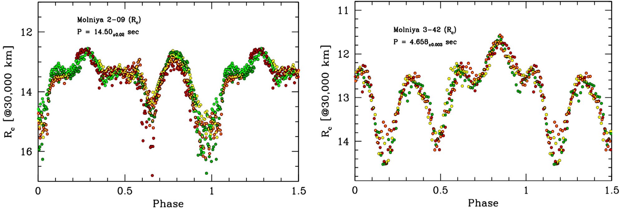 |
Figure 6 -
The R-band lightcurve of Molniya 209 (left) and 342 (right), respectively as from Cananea observations of 2015
September 20 and Loiano 2014 October 17. The same pattern can easily be recognized in both plots, as a sort of bona
fide photometric signature of Molniya satellites.
|
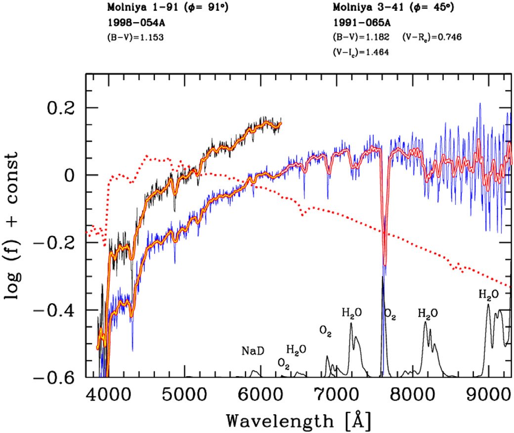 |
Figure 7 -
The reflectance spectra of Molniya 191 (black curve) and 341 (blue curve), as from BFOSC spectroscopic observations
in Loiano. Molniya 191 has been observed through grism GR3, while Molniya 341 data are from the GR3+GR5 combination
(R~400). Both spectra have been smoothed (yellow- red moving average on the plots) for better display. The solar spectrum
is overplotted (within arbitrary offset), for comparison (red dotted curve). The absorption features in the satellite
spectra are due to the Sun or the telluric absorptions, in the near infrared, mainly by water vapor and Oxygen, as singled
out in the lower sketch. Note the fairly reddish color of both Molniyas, compared to the Sun.
|
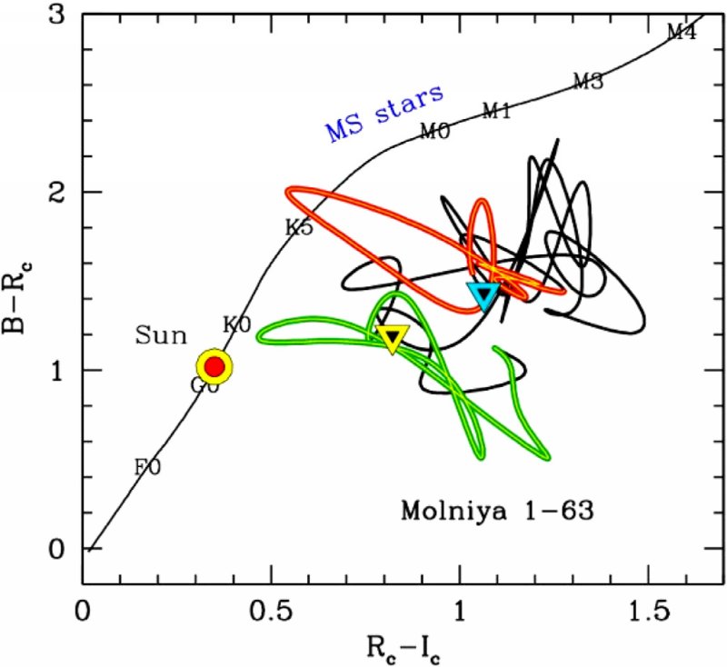 |
Figure 8 -
The observed color path of Molniya 163 along its rotation, as from the 2016 Loiano observations (see Fig. 5,
right panel) in the (Rc−Ic) vs. (B−Rc) diagram. The lightcurve maxima (that
is when solar pads are reflecting) are singled out in green (primary peak) and red (secondary peak), while the black line
mainly traces satellite bus reflectance. The big blue and yellow triangles mark respectively the time- and luminosity-averaged colors.
For comparison, the (Rc−Ic) vs. (B−Rc) locus for Main-Sequence
stars of different spectral type after [15] is also displayed on the plot, marking the Suns location.
|
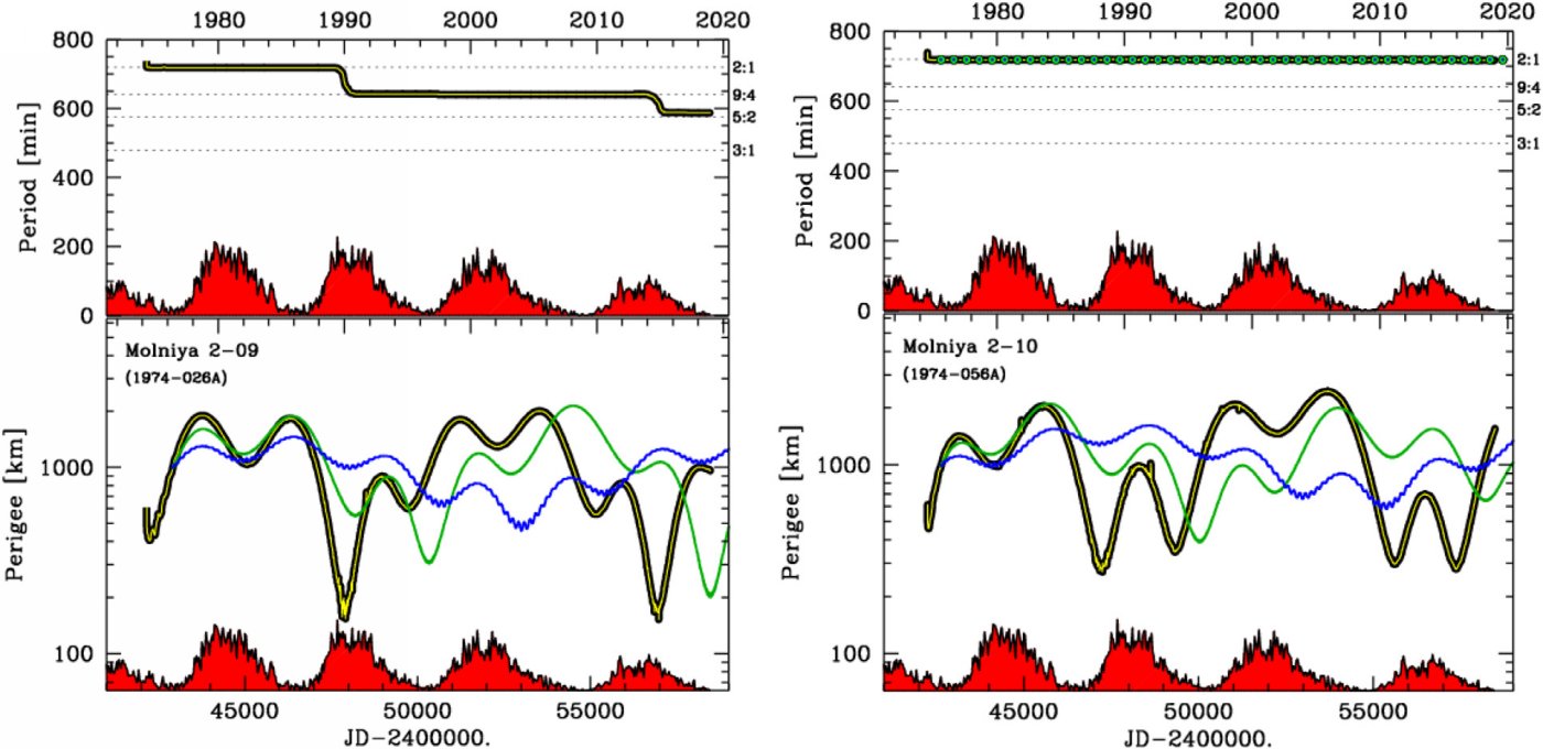 |
Figure 9 -
The historical track of Molniya 209 and 210, the two oldest satellites in orbit since 1974, are reported
according to [11]. Orbit evolution is assessed in terms of drag and lunisolar perturbation acting on the satellite
semi-major axis (taking period as a proxy) and eccentricity (with perigee altitude as a proxy). The FOP semi-analytical
orbital propagator [19] has been used for our analysis. The historical data are in black, while the Moon and Sun
perturbation is singled out, respectively by the green and blue curves and dots. Solar activity is sketched below in
each panel (red histogram). Note the 7.5, 11 and 24-yr breathing pulse on satellite eccentricity induced by the
lunisolar perturbation, as discussed in the text. For Molniya 209 notice as well the period switch, leaving the original
2:1 resonance during two deep excursions of perigee into the atmospheric drag, about year 1990 and 2015.
|
Back to article listing |
|
Shortcut to Space Stuff |
| AB/May 2021 |
|
|