Back to article listing

Back to article listing |
|
Shortcut to Space Stuff |
| Buzzoni, A.: |
| "Wide-Field Optical Tracking of LEO Objects: Theoretical Assessment and Observing Strategy" 2024, Advances in Space Research, 74, 4990 |
|
|
Summary:
The main technical and strategic aspects related to Space Surveillance and Tracking (SST) with optical
sensors are set in context in this study to lead to an efficient inventory of the active satellites and
un-cooperant space debris population at Low-Earth orbital regimes (LEO). In particular, special emphasis
is devoted to the combined interplay between timing of observations, target illumination conditions,
instrumental fine tuning and data acquisition mode (surveying vs. active tracking).
At LEO altitudes, satellites are seen to cross the sky at very high angular velocity, in excess to
0.5-1.5 deg/sec, always making their positional measurements (and the inferred dynamical properties)
a challenging task for ground telescopes. To this aim, objective criteria have to be identified for a
best trade-off between instrument field of viev (FOV), CCD/CMOS platescale, telescope aperture and exposure
time in order to maximize target(s) detection and reference grid of stars valuable for astrometry.
Many counter-intuitive aspects are discussed in this regard, compared for instance with a more classical
"astronomical" approach, delving in particular the widely recognized inherent link between time-tag
accuracy and resolving power of optical imagery to track LEO objects.
A number of tables and graphical plots are provided for practical use to the reader.
|
|
Enhanced HTML/PDF version at the Journal site (*) (*) May require access password |
Local link to a working PDF version (1.2 Mb) (For personal use only) |
|
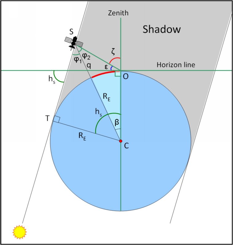
Figure 1 -
Apparent angular velocity, as seen from a ground observing station, for objects in prograde (yellow curve)
and retrograde (cyan curve) orbit, at high elevation above the horizon, as in eq. (2). The approximate relationship as
from eq. (3) is also displayed (green points and curve).
|
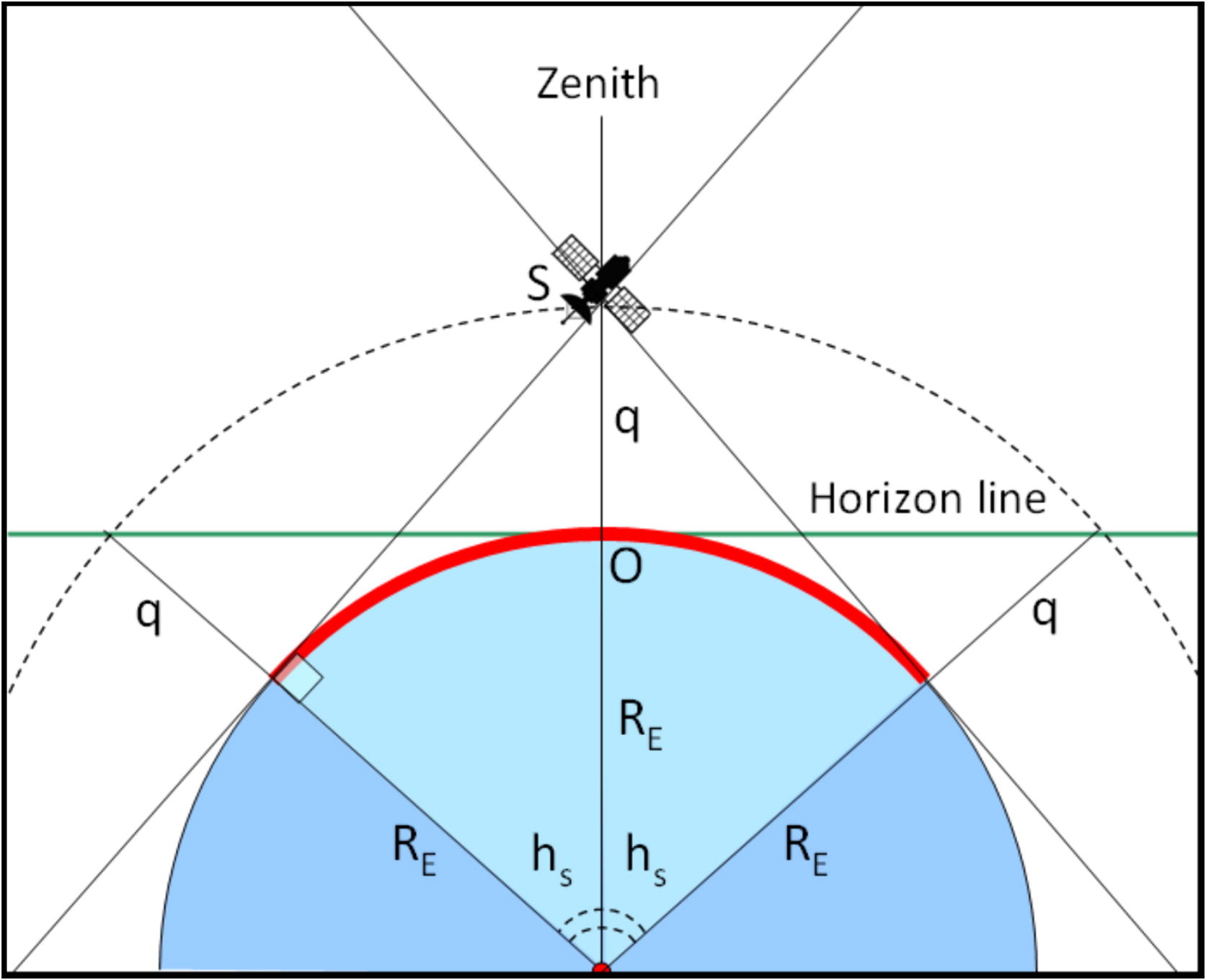
| Figure 2 -
The geometric reference for the visibility horizon (red arc) from a satellite orbiting at an altitude "q".
|
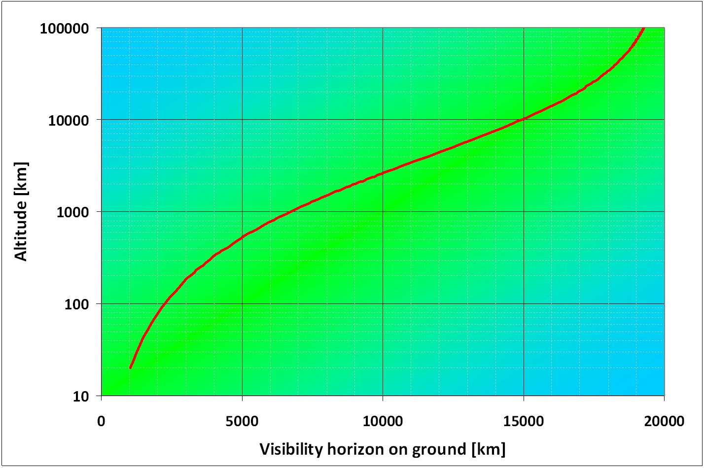 |
Figure 3 -
The satellite visibility horizon for orbits at different altitude. Note that the horizon tends asymptotically to the whole
hemisphere πRE ~20,000 km when the satellite moves very far away from Earth.
|
|
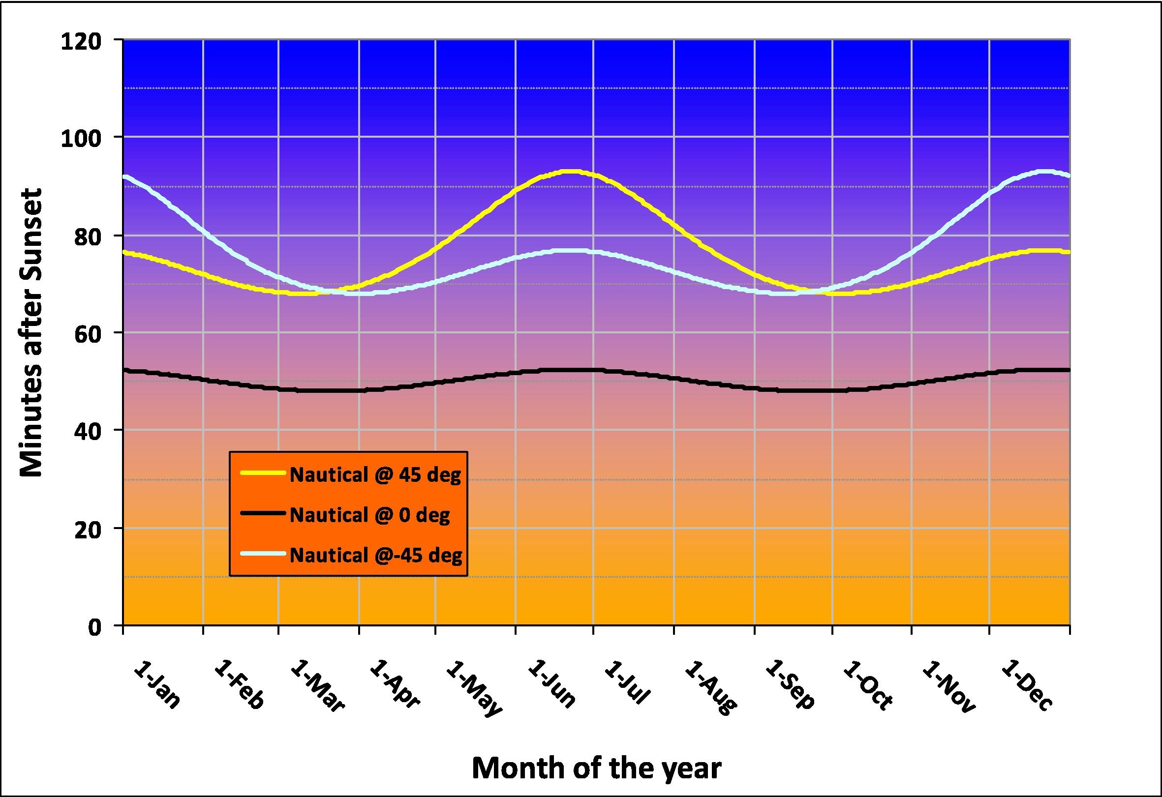
Figure 4 -
The Nautical Twilight circumstance, in minutes after the local sunset (or before the dawn) for an observer located at the
equator (black line) or at mid-latitude in the Northern (yellow line) and Southern (cyan line) hemisphere. The Nautical Twilight
instant may set the start of SST optical observations.
|
 |
Figure 5 -
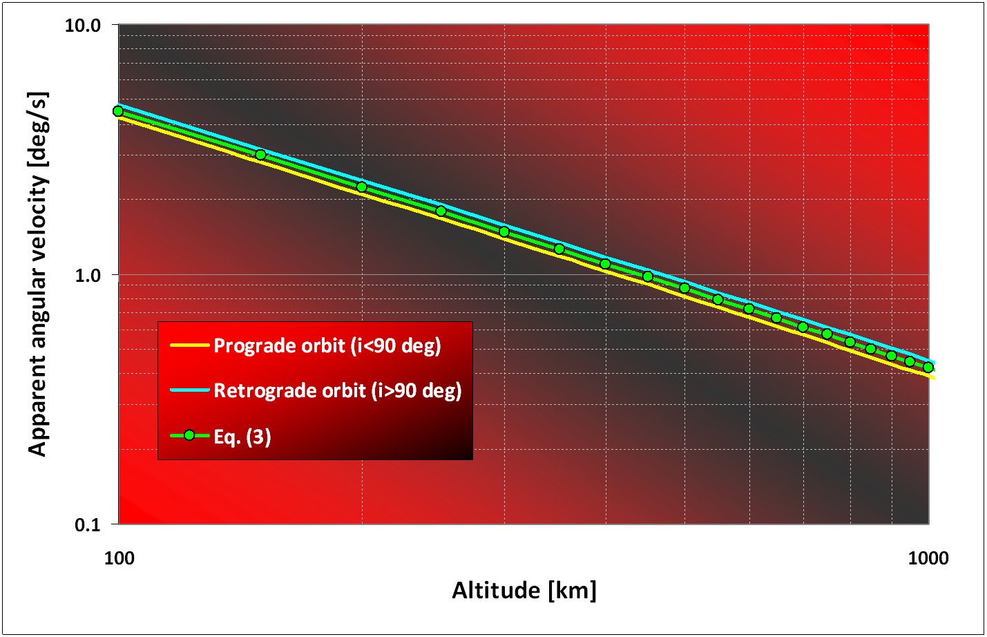
The geometric reference for the shadowing conditions of a satellite "S" orbiting at an altitude "q",
as seen from an observer "O" at a zenith angle ζ.
|
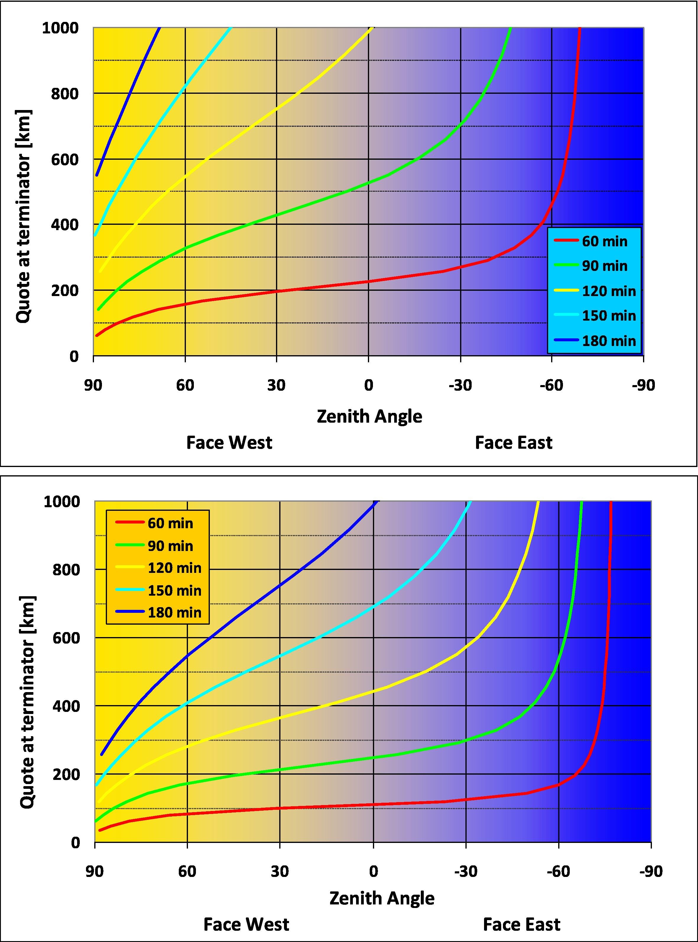 |
Figure 6 -
The quote and zenith angle of Earth's shadow terminator along the night for two observers located at the Equator (upper panel)
and at λ= 45o (lower panel) around the solstice seasons (i.e. Mar-Apr and Sep-Oct). The relevant relationship
is given for different time delays in minutes after the local sunset (or before the local dawn), by matching eq. (8) and (7),
as displayed in the inset legend. Orbiting objects are sunlit only left to each curve. For the beginning of night, zenith-angle
notation assumes positive values when looking West and negative values "face East". The opposite is true for the dawn observations.
|
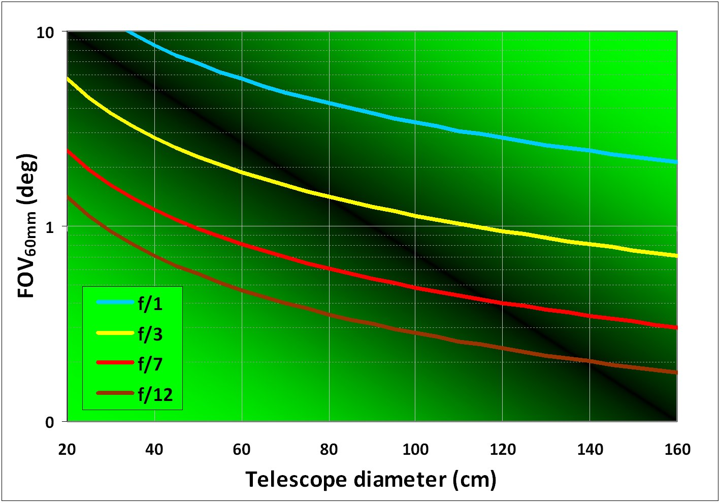 |
Figure 7 -
The projected FOV on a Medium Format (60 × 60 mm) CMOS, for telescopes of different size and relative aperture (f-number).
|
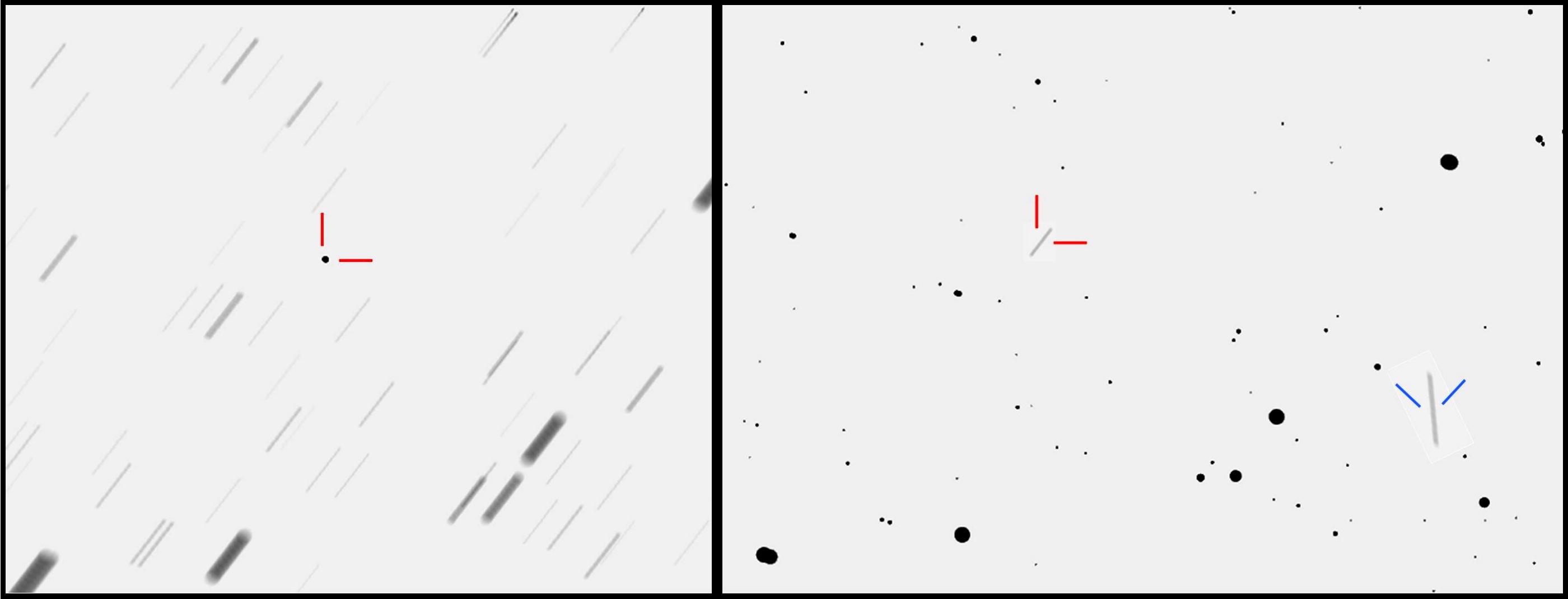 |
Figure 8 -
An illustrative sketch of the tracking (left panel) vs. surveying (right panel) strategy. Shallower stars and an enhanced
target signal (red markers) is secured by docking the object, like in the left panel. However, as stars trail across the
field, most of them (all those which totally or partially overspill del FOV borders) end up to be useless for any astrometric
calibration. In addition, by focussing on the envisaged target, the tracking telescope looses a serendipitous intruder
(trailing in the right panel and marked in blue) which, on the contrary, is caught by the surveying sensor.
|
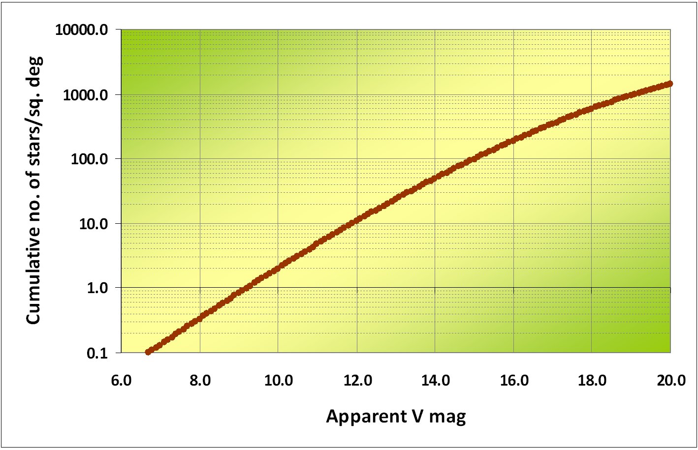 |
Figure 9 -
Cumulative star counts per square degree, with increasing apparent V magnitude, at the North Galactic Pole according to the
Bahcall & Soneira (1980) model.
|
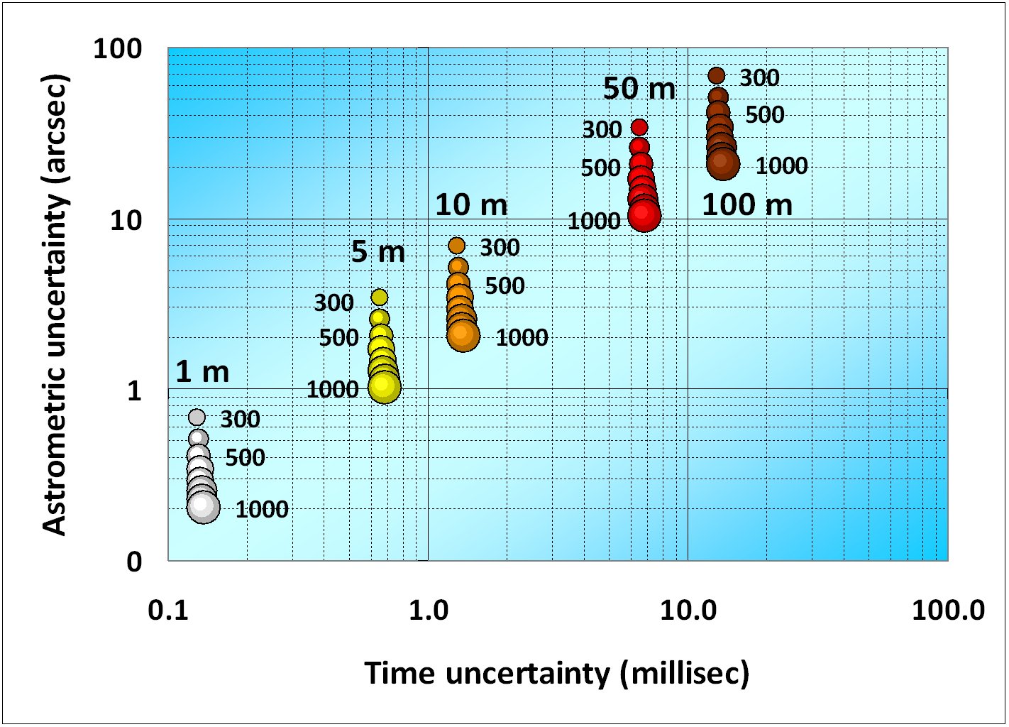 |
Figure 10 -
A comparison of the required accuracy for astrometry and time tag to reach the same absolute metric accuracy in target colocation
along its orbit. Each point sequence is labelled according to the LEO quote, from 300 to 1000 km. White dots refer to an
absolute accuracy of 1 meter in space, yellow dots are for 5 meters, orange points for 10 meters, red dots for a 50 meters and
finally brown markers are for a 100 meters absolute uncertainty. Note that required accuracy figures for time tag of observations
(milliseconds or so) far exceed the standard astrometric performance in the target measurements (arcseconds or so).
|
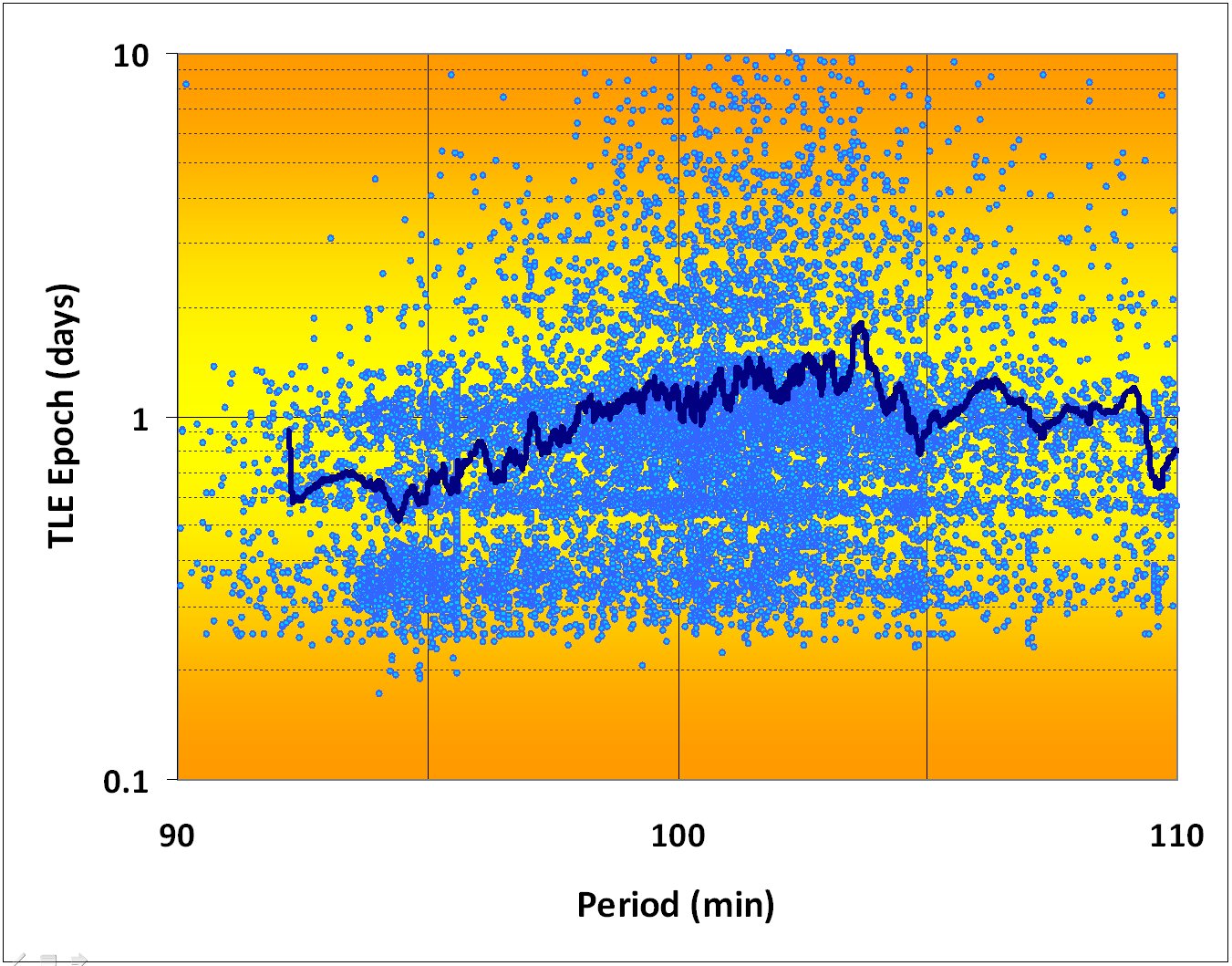 |
Figure 11 -
The epoch distribution of an illustrative sample of the NORAD/Celestrak TLE database for the LEO population according to the
orbital period in minutes. About 15,000 objects are displayed in the plot, within a 110 min period. Superposed (black curve)
is a moving average over 200 points. Note that for most of the objects the orbit is refreshed once (or even twice) a day.
|
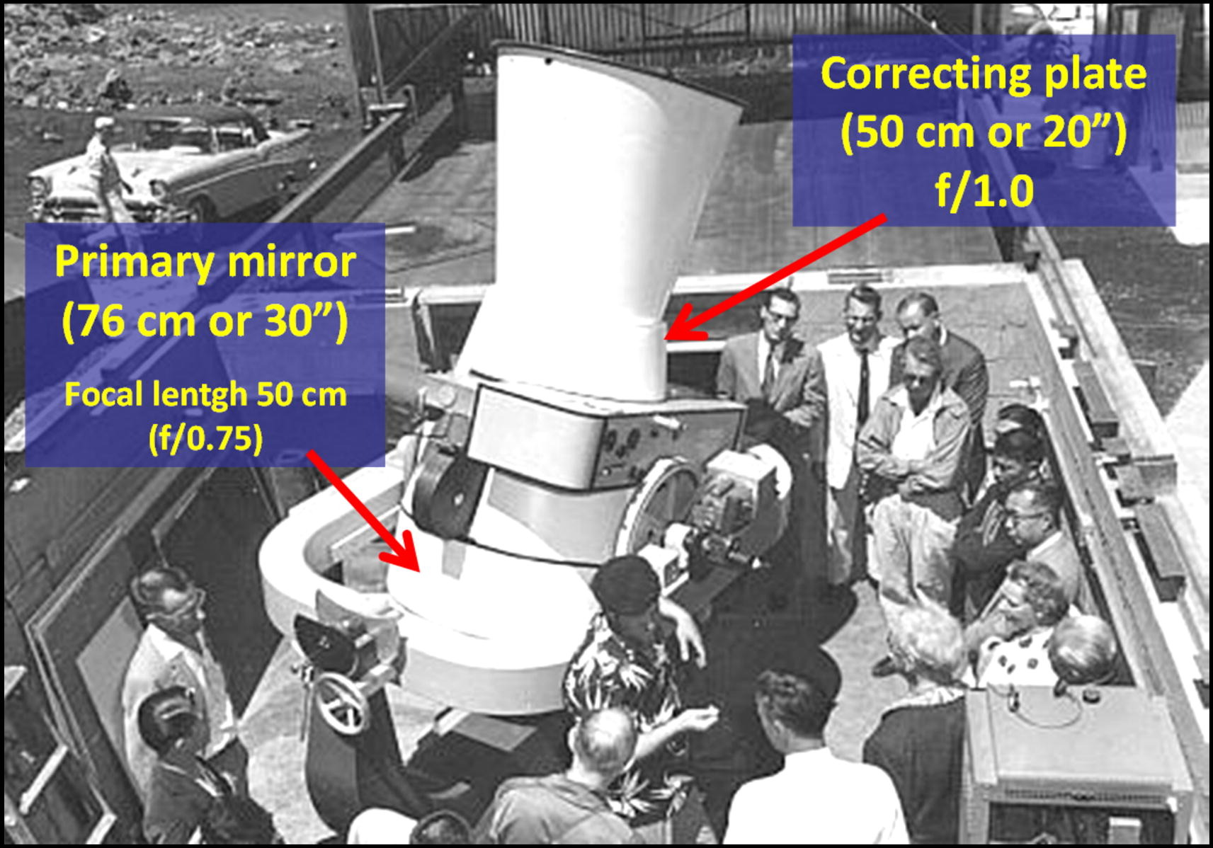 |
Figure 12 -
The SAO Baker-Nunn camera for satellite tracking, one out of a total of 17 worldwide stations, was dedicated on Aug 2, 1958 at
the Haleakala Hawaiian observatory. The main optical features of this telescope are marked in the figure. In particular, we
recognize the 76 cm primary mirror and the 50 cm correcting plate, which offered a relative aperture of f/1 for the whole instrument.
The original image is courtesy of Prof. Walter Steiger. The unannotated image is available at
this URL.
|
| Tables | |
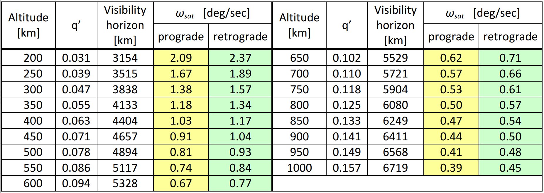 |
Table 1 -
Apparent zenith angular velocity and visibility horizon for objects in LEO orbit.
|
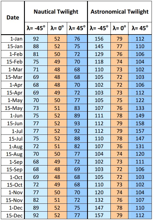 |
Table 2 -
Nautical and Astronomical Twilight instants, in minutes after the local sunset (or before the dawn) for an observer located at the equator
(λ = 0o) or at mid-latitude in the Northern (λ = +45o) and Southern (λ=−45o) hemisphere.
|
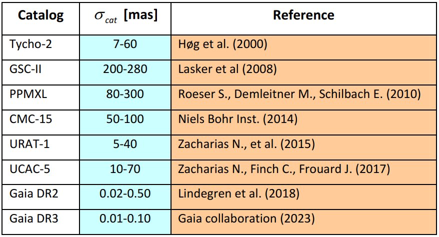 |
Table 3 -
Positional uncertainties of different reference star catalogs for astrometric applications.
|
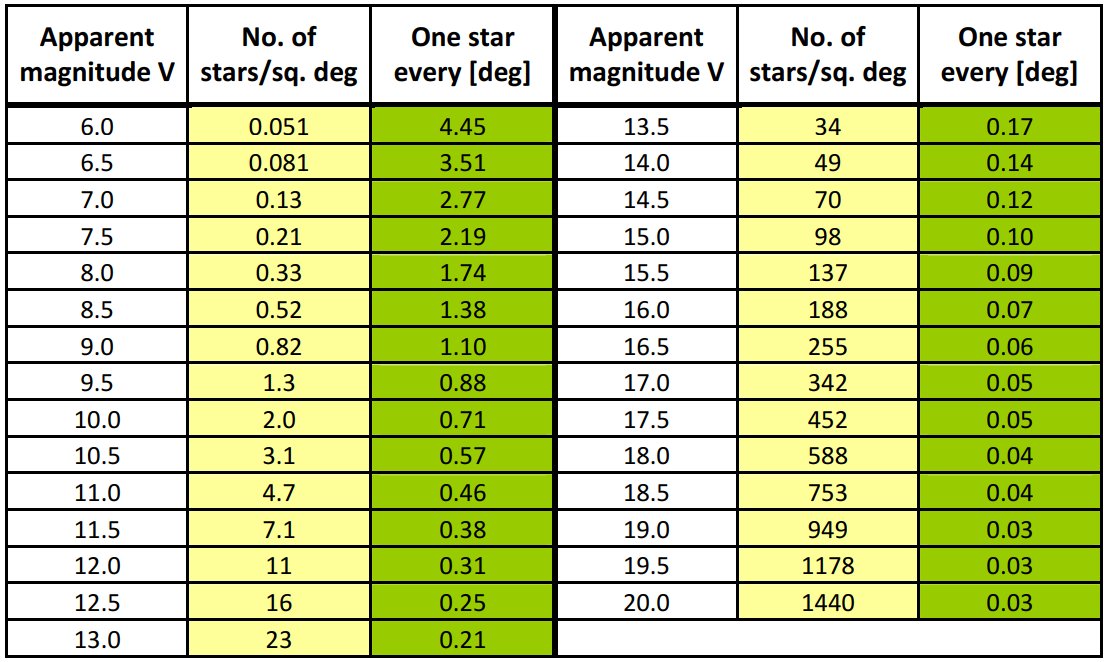 |
Table 4 -
Cumulative star counts per square degree, with increasing apparent V magnitude, at the North Galactic Pole according to the
Bahcall & Soneira (1980) model.
|
Back to article listing |
|
Shortcut to Space Stuff |
| AB/Nov 2024 |
|
|