| Saracco, P., D'Odorico, S., Moorwood, A., Buzzoni, A., Cuby, J.G., Lidman, C.: |
| "IR colors and sizes of faint galaxies", |
| 1999, Astron. Astrophys., 349, 751. |
 ASCII file ASCII file
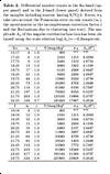
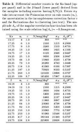
| Table 2 -
Differential number counts in the Ks-band (upper panel)
and in the J-band (lower panel) derived from the samples including
sources having S/N ≥ 5.
Errors σ _N take into account the Poissonian error on raw counts (n_r),
the uncertainties in the incompleteness correction factor "c" and the
fluctuations due to clustering (see text). The amplitude A_ω of the
angular correlation function has been obtained using the scale relation
log(A_ω )~ -0.3 mag+cost. |
 ASCII file ASCII file
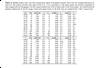
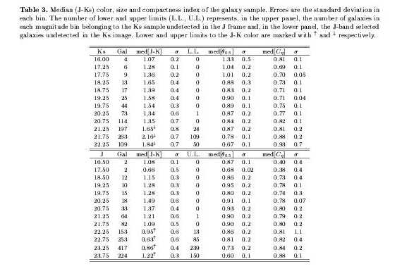
| Table 3 -
Median (J-Ks) color, size and compactness index
of the galaxy sample. Errors are the standard deviation in
each bin. The number of lower and upper limits (L.L., U.L.)
represents, in the upper panel, the number of galaxies in each magnitude bin
belonging to the Ks sample undetected in the J frame and, in the lower panel,
the J-band selected galaxies undetected in the Ks image.
Lower and upper limits to the J-K color are marked with ↑
and ↓ respectively. |
 ASCII file ASCII file
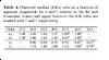
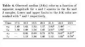
| Table 4 -
Observed median (J-Ks) color as a function of apparent magnitude for
"s" and "l" sources in the Ks and J samples.
Lower and upper limits to the J-K color are marked with ↑
and ↓ respectively. |
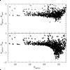
| Figure 1 -
Differences between the magnitude estimates for the Ks selected
sample:(upper panel) difference between aperture corrected magnitude
(K_ApCorr) and AUTO (Kron-like) magnitude (K_Auto); (lower panel)
difference between aperture corrected magnitude and isophotal magnitude
(K_Iso). The aperture correction (0.25 mag) between 2.5" and 5"
has been obtained using a sample of sources brighter than Ks =18.5. |
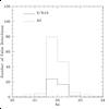
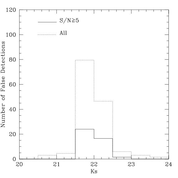
| Figure 2 -
Distribution of spurious sources. The dotted histogram
refers to the distribution of detections with minimum S/N =2.2
within the seeing disk. The thick line describe the distribution
of detections having S/N ≥ 5. |
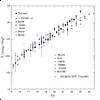
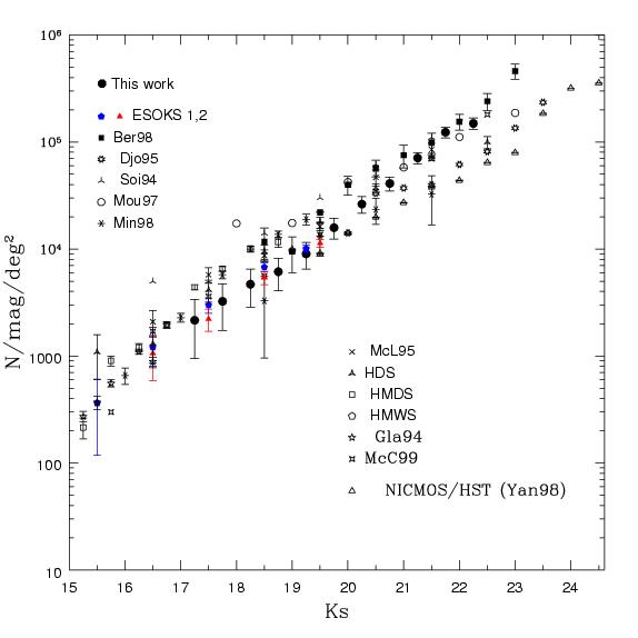
| Figure 3 -
The figure compares the Ks-band counts obtained in this
work with those in the literature:
Djorgovski et al. (1995, Djo95), Bershady et al. (1998, Ber98)
(obtained at the Keck telescope), Gardner et al. (1993, HMWS, HMDS, HDS),
Glazebrook et al. (1994, Gla94), Soifer et al. (1994, Soi94),
McLeod et al. (1995, McL95), Moustakas et al. (1997, Mou97),
Saracco et al. (1997, ESOKS1, 2), Minezaki et al. (1998, Min98) and
McCracken et al. (1999, McC99).
NICMOS/HST H-band counts of Yan et al. (1998, Yan98) are also shown.
The slope of our counts (~0.38) agree very well with those obtained
by McL95, Djo95 and Ber98 while it is significantly steeper than
the slope obtained by Gardner et al. (1993) and by Mou97. |
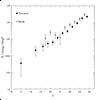
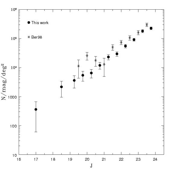
| Figure 4 -
The J-band galaxy counts obtained in this work are
compared with those previously obtained by Bershady et al. (1998, Ber98).
The J-band counts continue to rise with a power law slope of ~0.36
showing no signs of flattening down to J = 24.0. |
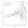
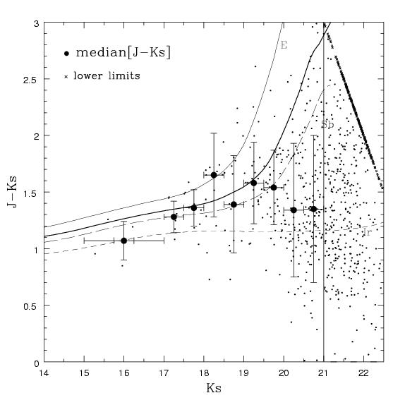
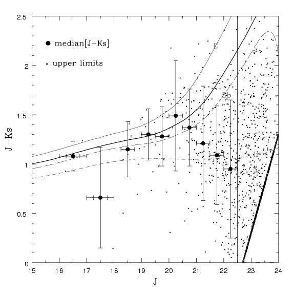
| Figure 5 -
Color-magnitude diagram of our Ks galaxy sample.
Large filled points represent the median J-Ks color.
Vertical error bars are the standard deviation from the mean.
The bin widths (usually 0.5 mag) are represented by the horizontal bars.
Small crosses mark undetected J galaxies, i.e. the J-Ks lower limits.
The vertical straight line represents the completeness J-band detection limit
for the Ks sample. The thick solid curve is the expected apparent color of a local galaxy
mix (see Sec. 6.2 and Tab. 4) evolved back
to high redshift (z > 10) according to the models of Buzzoni (1998).
The expected J-K color for a pure galaxy population of E (thin solid line),
Sb (long-dashed line) and Im (short-dashed line) types is also
reported as labeled in the figure. Models assume a
(H_o, q_o = 50, 0.5) cosmology. |

| Figure 6 -
Same as Fig. 5 but for the J-selected galaxies.
The vertical solid line indicates the detection limit of the J sample
in the Ks frame. |
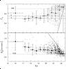
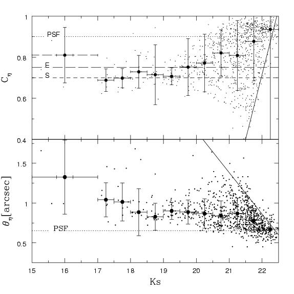
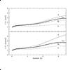
| Figure 7 -
Compactness index C_η (upper panel)
and apparent size θ _0.5 (lower panel) as a function of Ks magnitude.
The filled (red) circles are the median values in a 0.5 mag bin width.
Vertical error bars are the standard deviation in each magnitude bin
while horizontal bars represent the bin width.
The dotted, the dashed and the long-dashed lines in the upper panel
indicate the values of C_η for PSF, Spiral and Elliptical profiles
respectively (see Sec. 5.2).
The solid line in the lower panel shows the magnitude enclosed in
an aperture of radius θ and a uniform surface brightness
Ks = 22.76 mag/sqarcsec while the dotted line represent the characteristic
size of a point source in our images. |
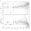
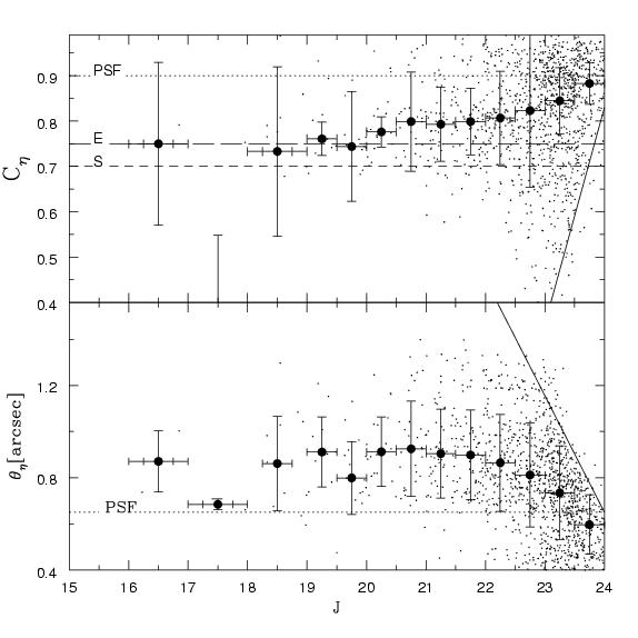
| Figure 8 -
Same as in Fig. 7 but for the J sample.
The solid line in the lower panel shows the magnitude enclosed in
an aperture of radius θ and a uniform surface brightness of
J=23.88 mag/sqarcsec. |
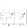
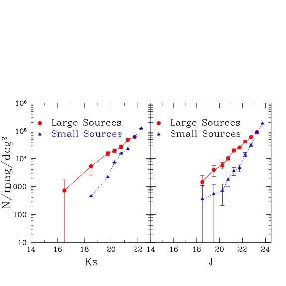
| Figure 9 -
Ks-band (left) and J-band (right) differential number counts
for small and large galaxies: small galaxies are those having
θ (K_0.5) ≤ 0.79 arcsec and θ (J_0.5) ≤ 0.73 arcsec.
The slope of the counts are γ **s_Ks ~ 0.6
and γ **s_J ~ 0.56 for small sources and γ **l_Ks ~ 0.36 and
γ **l_J ~ 0.38 for large sources. |
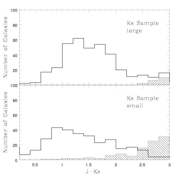
| Figure 10 -
J-Ks color distributions (thik histograms) for "l"
(upper panel) and "s" sources (lower panel) belonging to the Ks sample.
The shaded histograms represent the distribution of the J-Ks
lower limits i.e. galaxies redder than J_lim − Ks (J_lim) = 24.8, Sec. 4.2). |

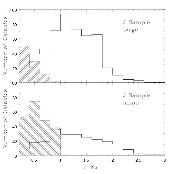
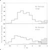
| Figure 11 -
J-Ks color distribution for "l" (upper panel) and
"s" sources (lower panel) belonging to the J sample.
The shaded histograms represent the distribution of the J-Ks
upper limits i.e. galaxies bluer than J-Ks_lim (Ks_lim = 23.05, Sec. 4.2). |
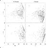
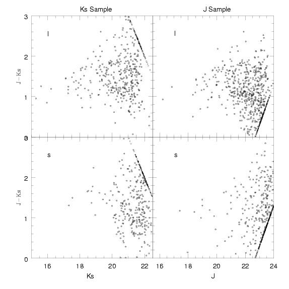
| Figure 12 -
Color-magnitude diagram of "s" (lower panel)
and "l" (upper panel) sources for Ks sample (left) and J sample (right). |
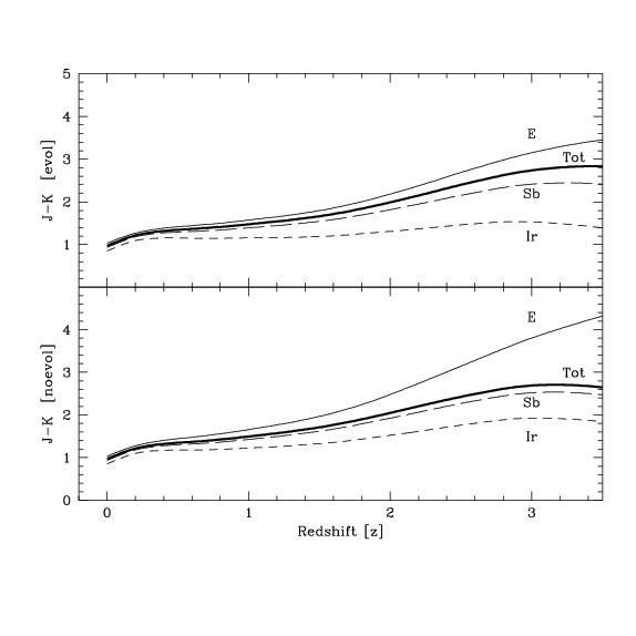
| Figure 13 -
Expected J-Ks color of different galaxy types as a function
of redshift in the case of no-evolution (lower panel) and
evolution (upper panel). The mean expected color of the local galaxy
mix as in Marzke et al. (1998) is also shown (thick solid line). |

 ASCII file
 ASCII file
 ASCII file