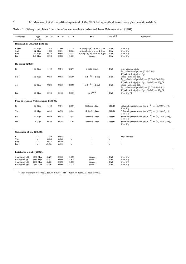
| Table 1 - Galaxy templates from the reference synthesis codes and from Coleman et al. (1980) |

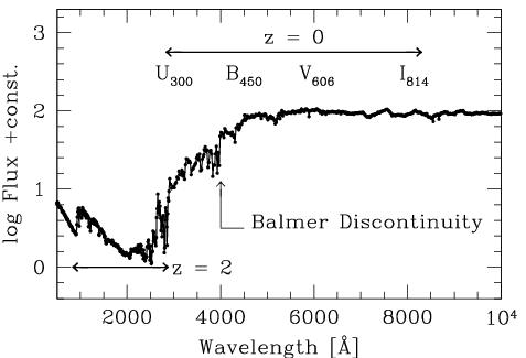
| Figure 1 - Restframe portion of galaxy SED explored by the WFPC2
photometric system at z = 0 and z = 2. As an illustrative example
a template model for local elliptical galaxies is shown. |
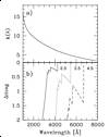
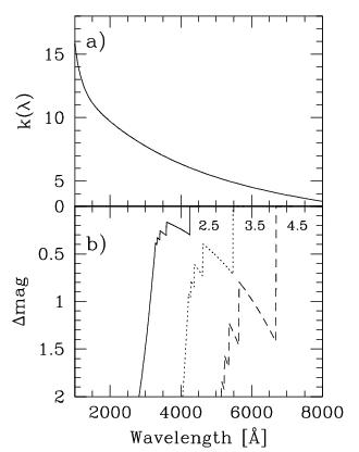
| Figure 2 - Panel a: the adopted dust attenuation law after
Calzetti (1999). Panel b: the IGM attenuation in a magnitude
scale at redshift 2.5, 3.5 and 4.5, as labelled, according to Madau (1995). |
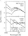
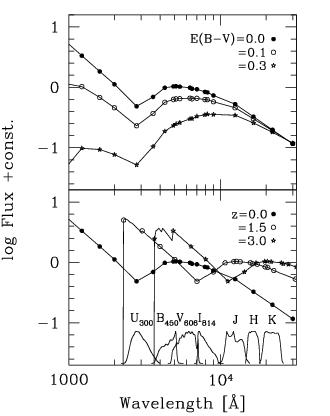
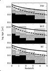
| Figure 3 - The effect of internal reddening and IGM on the Sb reference
template from Buzzoni (2000). Dust attenuation for E(B−V) up to 0.3
mag, as labelled, is shown in the upper panel, while the expected
break induced by the Ly-α forest at z = 1.5 and z = 3 is
shown in the lower panel. For reference, the HST photometric
system and the Johnson JHK bands are displayed at the bottom. |
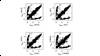
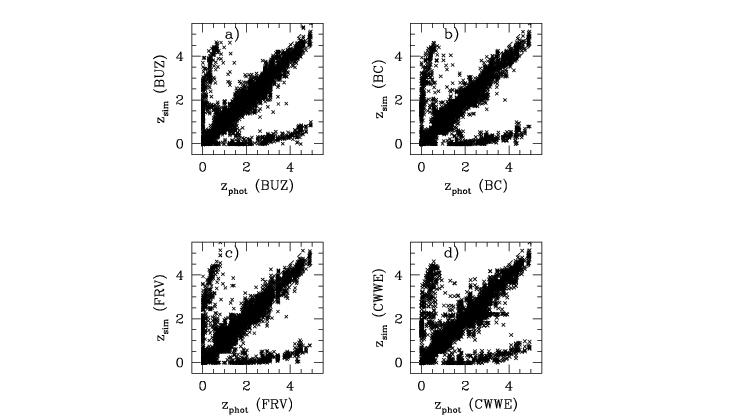
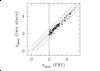
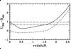
| Figure 4 - Comparison of the statistical uncertainty in the redshift
estimate due to photometric errors for the BC, BUZ and FRV reference
libraries, as well as for the CWWE empirical templates. Residuals are
from a bootstrap simulation of the FSLY galaxy catalog (1041 objects
for each of ten simulated catalog samples). |
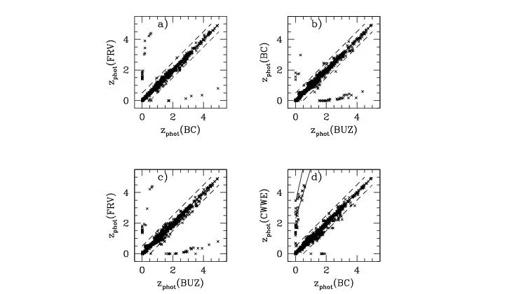
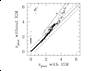
| Figure 5 - Comparison of HDFN expected redshift distribution, for
different reference libraries. The solid line is for Δ z = 0.0,
while long-dashed strip is for Δ z = ± 0.5. The vertical
strip (solid lines) in panel (d) encloses the catastrophic
outliers coming from the misinterpretation of the Balmer/Lyman break
(see text for further details). |
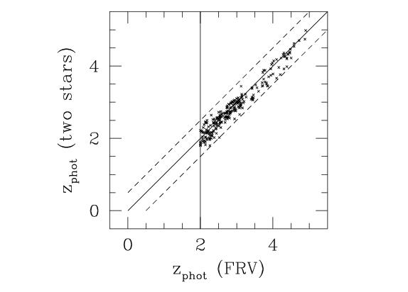
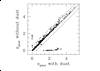
| Figure 6 - SED fitting of the FSLY galaxy subsample beyond z > 2. The
data distribution by matching the FRV template set is compared with a
"minimal" reference library consisting of two Kurucz' (1992) model
atmospheres for stars of spectral type B0 and B2. The relative
σ(z) results 0.18 with no apparent drift in the data
distribution. The solid line is for Δ z = 0.0, while
long-dashed strip is for Δ z = ± 0.5. See text for a full
discussion. |
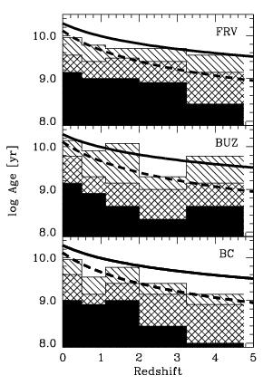
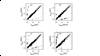
| Figure 7 - The expected age-redshift relation from the BC, BUZ and FRV
best templates by imposing no cosmological constraint. HDFN galaxies
have been grouped in order to guarantee at least 100 objects per
redshift bin. Solid, grid, and diagonal-shaded histograms are the
50%, 75%, and 90% envelopes of galaxy age distribution. In each
plot, solid and dotted lines are the theoretical age-z relation for
H_o = 50 and q_o = 0.0 and 0.5, respectively. |
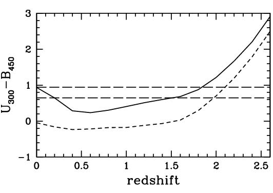
| Figure 8 - The U_300−B_450 apparent color as a function of
redshift for the CWW Im empirical template (solid line) and
Leitherer et al. (1999) 50 Myr starburst model (dashed line). In
absence of any starburst template, a fraction of star-forming
galaxies at z ~ 2 (with U_300−B_450 ~ 0.8) might be
interpreted as local (z ≤ 0.2) irregulars. |
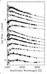
| Figure 9 - Restframe composite SED from the HST data for the 341 HDFN
galaxies with fiducial z > 1.5 compared with the CWWE reference
templates. From top to bottom solid lines display the starburst
template with t = 500 Myr and E(B−V) = 0.0, 0.05, 0.1, 0.2, 0.3, the t =
50 Myr starburst model with E(B−V) = 0.0, 0.05, 0.1, 0.2, 0.3, the Scd
and the Im CWW spectra. |
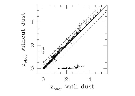
| Figure 10 - The selective influence of galaxy internal reddening on the
SED fitting performance. The HDFN redshift distribution from the BC
template set is displayed with and without taking into account for ISM
absorption. This is done by leaving E(B−V) = 0 or as a free fitting
parameter in the range 0.0 ≤ E(B−V) ≤ 0.3. Long-dashed lines
in the plot represent Δ z = ± 0.5. |
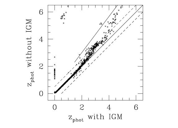
| Figure 11 - Comparison of the HDFN redshift distribution obtained from
the BUZ reference library with and without taking into account the IGM
absorption. Long-dashed lines in the plot represent Δ z = ± 0.5.
The solid line shows the expected upper limit in the
redshift drift due to the the misinterpretation of the intrinsic Lyman
break with the Ly-α forest effect. |