Whole ASCII file
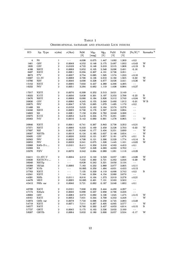
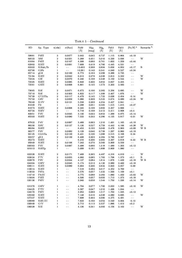
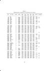
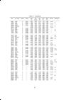
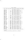
| Table 1 -
Observational database and standard Lick indices. |
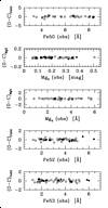
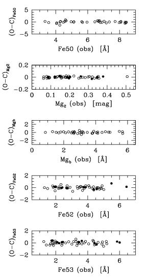
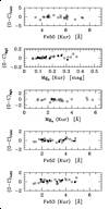
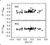
| Figure 1 -
Index calibration to the standard Lick system. Residuals for
the 36 primary calibrators (of luminosity class V-IV-III) in common with
W94 (ο) and a "check sample" of 13 stars in common with B92 and B94
(•) are displayed, after application of eq. (4). Point
scatter is σ(Fe50) = ± 0.39 Å, σ(Mg_2)
= ± 0.012 mag, σ(Mgb) = ± 0.19 Å, σ(Fe52) = ± 0.24 Å,
and σ(Fe53) = ± 0.25 Å. These values are comparable with the internal
uncertainty in the observations confirming the reliability of the
calibration procedure.
|
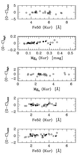
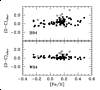
| Figure 2 -
Index calibration to the standard Lick system, after
eq. (4), for the fiducial model atmospheres of the 25 primary
calibrators in common with W94 (ο) and the 9 stars from
B92 and B94 (•). The (O − C) residuals are in the
sense [Synthetic -- Standard]. Point scatter
is σ(Fe50) = ± 0.70 Å, σ(Mg_2)
= ± 0.029 mag, σ(Mgb) = ± 0.40 Å,
σ(Fe52) = ± 0.27 Å, and σ(Fe53)
= ± 0.34 Å. These higher values, compared with
those of the observations (cf. Fig. 1), give a measure of the
residual variance of the theoretical models due to the intrinsic limitation
of the input physics. |
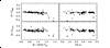
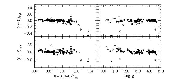
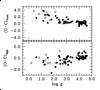
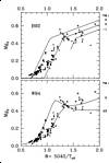
| Figure 3 -
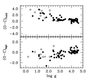
The (O − C) index residuals (in the sense [Observed − Synthetic])
for Mg_2 and combined Iron index are displayed vs. atmosphere
fiducial parameters Θ = 5040/T_eff
and surface gravity. Solid dots mark the "fair sample" of 73 stars
while open dots include the supplementary 18 stars with less confident
atmosphere match. As expected, the four coolest stars in the sample
(T_eff ≤ 4000 K) are poorly matched by the models while the remaining
point distribution is consistent with a zero-average residual. These four
outliers will not enter any further analysis. |
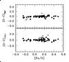
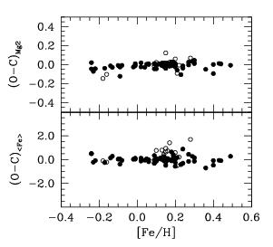
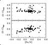
| Figure 4 -
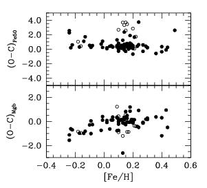
The metallicity scale is explored vs. (O − C) index residuals
(in the sense [Observed − Synthetic]) like in Fig. 3.
No (O − C) trend is found vs. [Fe/H], with index
residual distribution consistent with a zero average. At least 6 stars
can be confidently recognized with [Fe/H] in excess of +0.35 dex. |
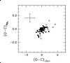
| Figure 5 -
The Mg_2 and index residuals between observations
and fiducial synthetic spectra are displayed for the "fair" (•)
and the "extended" (ο) sample.
The typical 2-σ error box of individual observations is displayed
top left in the figure. The lack of any clear anti-correlated
trend between the (O − C) residuals indicates, on the average, a solar [Mg/Fe]
relative abundance. See text for discussion. |
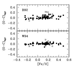
| Figure 6 -
The Mg_2 index residuals (in the sense [Observed − Computed])
with respect to B92 and W94
fitting functions vs. metallicity for the "fair" (•)
and the "extended" (ο) samples. Both (O − C) distributions are
consistent with a zero average. Point spread for the "fair" sample across
the B92 fitting function is σ(Mg_2) = ± 0.049 mag,
and σ(Mg_2) = ± 0.031 mag with respect to W94. |
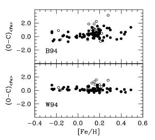
| Figure 7 -
Same as for Fig. 6 but for the combined Fe index
= (Fe52 + Fe53)/2.
Point spread of the "fair sample" (•) with respect to the
zero-average (O − C) is σ(< Fe >) = ± 0.61 Å comparing with
B94, and σ(< Fe >) = ± 0.30 Å with respect to W94. |
| Figure 8 -
Same as for Fig. 6 but for the Fe50 and Mgb indices.
The (O − C) residuals are computed with respect to the W94 fitting functions.
Point spread for the "fair sample" (•)
with respect to the zero-average (O − C) is σ(Fe50) = ± 0.95 Å,
and σ(Mgb) = ± 0.83 Å. A trend with [Fe/H] (opposite
for Fe50 and Mgb) appears in the data. |
| Figure 9 -
The Fe50 and Mgb (O − C) residuals as from Fig. 8
is explored vs. stellar gravity. The drift in the data distribution indicates
that log g dependence is not fully accounted for by the W94
fitting functions. The residual variance is the main responsible for the poorer
match to the observations in Fig. 8. |
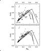
| Figure 10 -
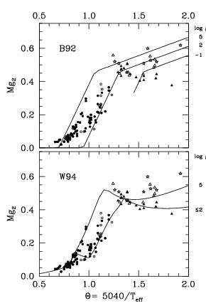
The Mg_2 data distribution (• = "fair", ο =
"extended" samples) vs. B92 and W94 fitting function predictions (solid lines).
To ease comparison, observations have been corrected to [Fe/H] = 0
by subtracting the corresponding [Fe/H] polynomial term of each fitting set.
In order to span the whole range of temperature, also Mg_2 measurements of
eight Gliese red dwarfs from B92 (star markers) have been added in both panels
together with ten M dwarfs from the Gorgas et al (1993) sample
(open triangles). The low-gravity range is also spanned by a set of 16 field M giants
with T_eff < 3900 K, from W94 (solid triangles). The B92 and W94 fitting
functions have been computed for log g = 5.0, 2.0 and -1.0 dex, as labelled in each
panel. Below 3900 K the W94 fit is insensitive to stellar gravity so that the
log g = 2 and -1 curves merge. A solar metallicity is assumed throughout in the
models. |
| Figure 11 -
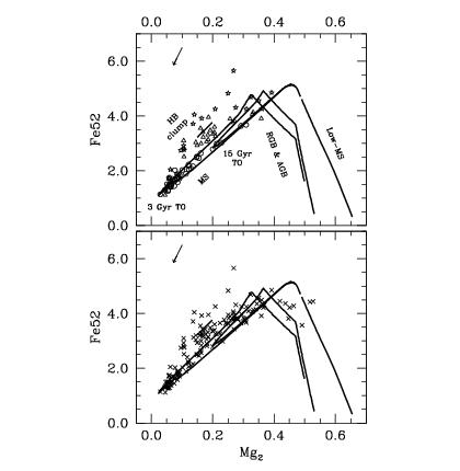
The Mg_2 vs. Fe52 distribution for the 87 stars with fiducial
atmosphere parameters in the "extended" sample (upper panel) and
for the global observed sample of 139 stars (lower panel).
Stars in the upper panel are marked according to their surface gravity
(stars: log g < 2.0; open triangles: 2.00 ≤ log g ≤ 3.5;
open dots: log g > 3.5).
The theoretical locus for a 3 and 15 Gyr old simple stellar populations
with [Fe/H] = +0.2 from Buzzoni (1989) is superposed
to the data, and main evolutionary
phases are labelled (MS = main sequence; TO = MS Turn off point;
RGB = red giant branch; AGB = asymptotic giant branch; HB = horizontal branch).
The vector top left in each panel is the expected variation in the observed
indices for a change in [Fe/H] of -0.5 dex. |