Back to article listing

Back to article listing |
|
Shortcut to Space Stuff |
| Alessi, E.M., Buzzoni, A., Daquin, J., Carbognani, A. & Tommei, G.: |
| "Dynamical properties of the Molniya satellite constellation: Long-term evolution of orbital eccentricity" 2021, Acta Astronautica, 179, 659 |
|
|
Summary:
The aim of this work is to analyze the orbital evolution of the mean eccentricity given by the Two-LineElements (TLE)
set of the Molniya satellites constellation. The approach is bottom-up, aiming at a synergy between the observed dynamics
and the mathematical modeling. Being the focus the long-term evolution of the eccentricity, the dynamical model adopted
is a doubly-averaged formulation of the third-body perturbation due to Sun and Moon, coupled with the oblateness effect on
the orientation of the satellite. The numerical evolution of the eccentricity, obtained by a two-degree-of-freedom time
dependent model assuming different orders in the series expansion of the third-body effect, is compared against the mean
evolution given by the TLE. The results show that, despite being highly elliptical orbits, the second order expansion catches
extremely well the behavior. Also, the lunisolar effect turns out to be non-negligible for the behavior of the longitude
of the ascending node and the argument of pericenter. Finally, a frequency series analysis is proposed to show the main
contributions that can be detected from the observational data.
|
|
Enhanced HTML/PDF version at the Ac&A site (*) (*) May require access password |
Local link to the PDF version (700 Kb)
(For personal use only) | ||
| Pick up the paper at Astro-ph/2007.04341 |
|
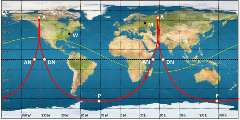
Figure 1 -
An illustrative example of Molniya orbit ground track. Two 12-hr orbits are displayed to span a full day.
The nominal orbital parameters are assumed, for illustrative scope, according to the template of Fortescue (1995).
In particular, for our specific choice, we set the relevant geometric orientation parameters
(i, ω) = (63.4o, 270o), with orbit
scale length parameters (in km) (a, hp, ha)km = (26560, 1000, 39360).
This implies an eccentricity e = 0.72 and a period P = 720 min. Note the extremely asymmetric
location of the ascending (AN) and descending (DN) nodes, due to the high eccentricity of the orbit, and the
perigee (P), always placed in the Southern hemisphere. Along the two daily apogees (A), the satellite hovers
first Russia and then Canada/US. The visibility horizon (aka the footprint) attained by the Molniya at its apogee
over Russia, is above the displayed yellow line. (For interpretation of the references to color in this figure legend,
the reader is referred to the web version of this article.)
|
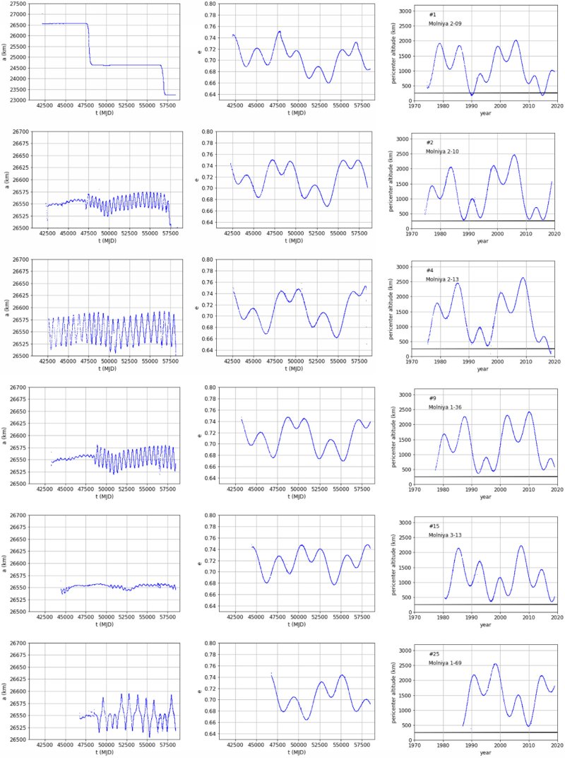
| Figure 2 -
Semi-major axis (left; km), eccentricity (middle) and pericenter altitude (right; km) mean evolution from
the TLE data of Molniya 2-09, 2-10, 2-13, 1-36, 3-13, 1-69 (#1, 2, 4, 9, 15, 25 of Table 1). On the right, the time
is displayed in decimal year for the sake of clarity; also, the black horizontal line highlights 250 km of altitude.
|
|
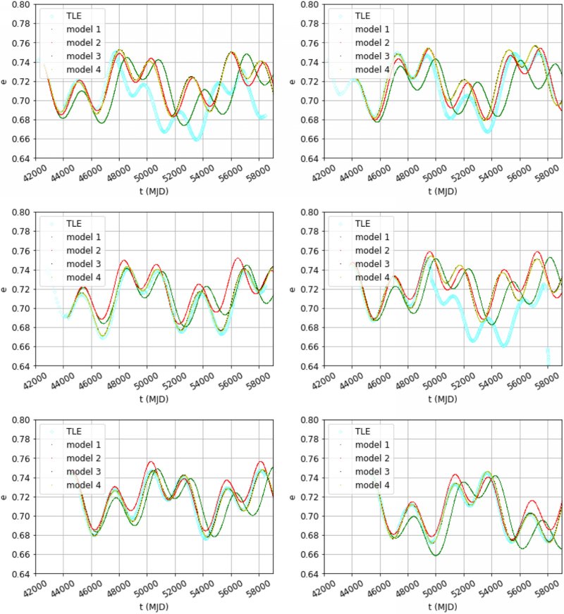
Figure 3 -
Eccentricity evolution obtained by assuming different levels of third-body perturbation of (e, i, Ω, ω),
compared against the TLE evolution for some specific examples. More details in the text. Top: orbits #1 and #2: middle: #7
and #13; bottom: #15 and #19. All the other orbits are shown in the SUPPLEMENTARY MATERIAL 2. The TLE evolution is displayed
in cyan; the evolution obtained by applying model 1 in green; the evolution obtained by applying model 2 in red;
the evolution obtained by applying model 3 in black; the evolution obtained by applying model 4 in yellow.
(For interpretation of the references to color in this figure legend, the reader is referred to the web version of this article.)
|
|
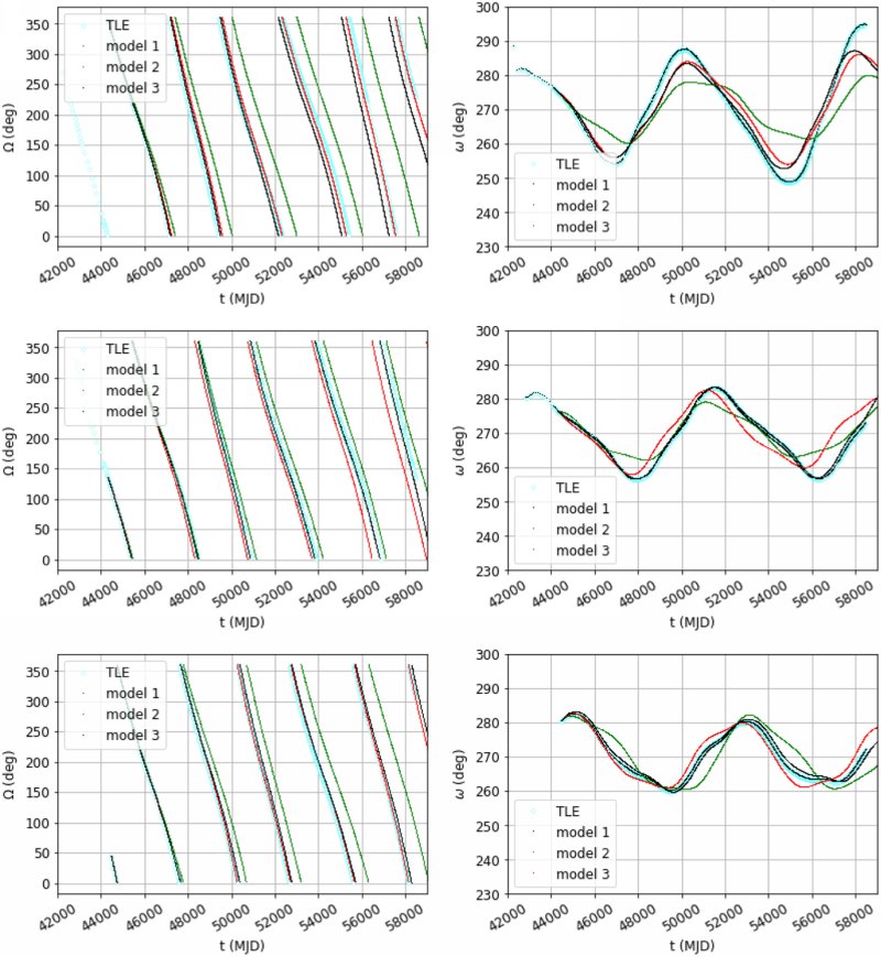
Figure 4 -
Longitude of the ascending node (left) and argument of pericenter evolution (right) evolution obtained by assuming
different levels of third-body perturbation of (e, i, Ω, ω), compared against the TLE evolution
for some specific examples.
More details in the text. Top: #2; middle: #7; bottom: #15. The TLE evolution is displayed in cyan; the evolution
obtained by applying model 1 in green; the evolution obtained by applying model 2 in red; the evolution obtained
by applying model 3 in black. (For interpretation of the references to color in this figure legend, the reader is
referred to the web version of this article.)
|
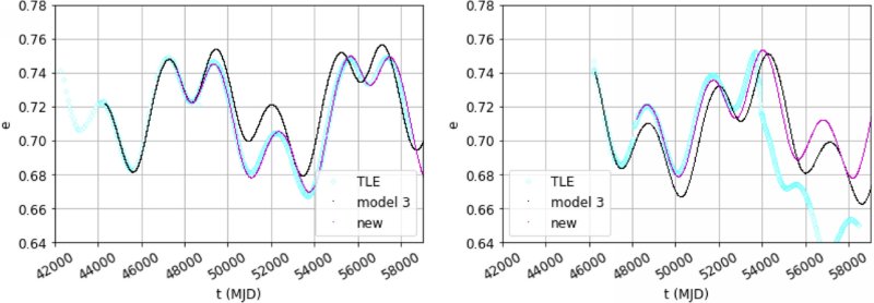 |
Figure 5 -
On the left, in cyan the eccentricity evolution of the TLE for Molniya 2-10 (orbit #2) and the ones obtained by numerical
propagation choosing two different initial conditions (black Table 1 and magenta Table 2). On the right, a similar experiment
performed for Molniya 3-24 (orbit #23). (For interpretation of the references to color in this figure legend, the reader is
referred to the web version of this article.)
|
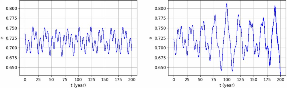 |
Figure 6 -
Propagation of 11 neighboring initial conditions, given the same initial epoch and using model 3. The initial conditions
have been taken from the propagation of the initial condition in Table 1, Table 2 for orbit #1 (left) and #2 (right),
respectively, by selecting the points xn = x(tn), tn = to + nΔt, n ∈ {−K, ..., K},
Δt = 1 day from the nominal trajectory. Such neighboring initial conditions are not
discernible the one from the other. The divergence among different orbits can be appreciable, but very slightly, only towards
of the end of the interval of propagation of Molniya 2-10 on the right. (For interpretation of the references to color in
this figure legend, the reader is referred to the web version of this article.)
|
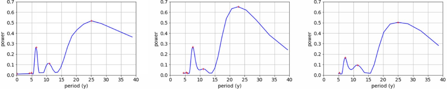 |
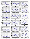
Figure 7 -
Example of the results obtained by applying a LombScargle procedure to the eccentricity series. From left to right:
Molniya 2-09, 2-10, 1-29 (orbit #1, 2, 3, respectively). In red, the dominant terms. (For interpretation of the references
to color in this figure legend, the reader is referred to the web version of this article.)
|
| Tables | |
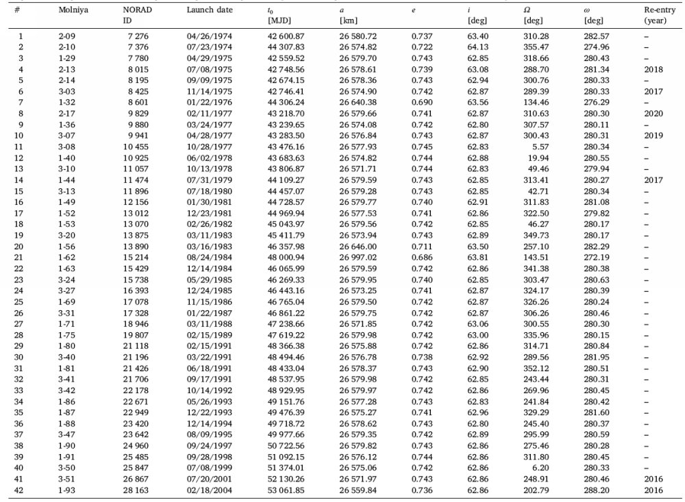 |
Table 1 -
Initial mean elements for the Molniya satellites considered. "#" identifies the sequential number of the orbit analyzed,
the second, the third and fourth columns report the official identification along with the launch date, to (MJD)
the initial epoch when the orbital elements are referred to, a is the semi-major axis (km), e the eccentricity,
ithe inclination (deg), Ω the longitude of the ascending node (deg), ω the argument of pericenter (deg).
On the choice of these initial conditions, please refer to the text.
|
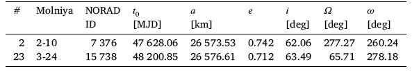 |
Table 2 -
Initial conditions for the evolution given in Fig.5.
|
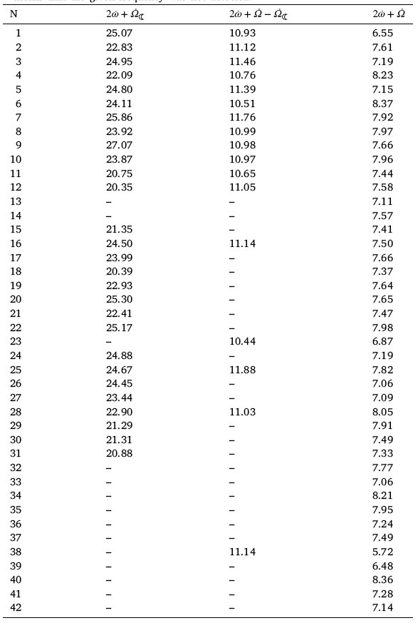 |
Table 3 -
Main periods (years) detected by means of the LombScargle procedure for each orbit. "−" means that the given frequency was not detected.
|
| Supplementary material | |
 |
S #1 -
In the following figures, we show the semi-major axis (left; km), eccentricity
(middle) and pericenter altitude (right; km) mean evolution from the TLE data
of the satellites reported in Tab. 1 of the main paper. On the right, the time
is displayed in decimal year for the sake of clarity. The black horizontal line on
the right plot highlights 250 km of altitude.
|
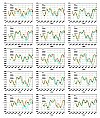 |
S #2 -
In the following figures, we show the eccentricity evolution obtained by assuming different levels of approximation
for the third-body perturbation in (e, i, Ω, ω), compared against the TLE evolution.
The color code is the following:
cyan: TLE evolution; green: evolution obtained by applying model 1; red: evolution obtained by applying model 2; black: evolution obtained by applying model 3; yellow: evolution obtained by applying model 4. Each plot corresponds to a satellite of Tab. 1 of the main paper. The ordering is left to right, top to bottom. |
Back to article listing |
|
Shortcut to Space Stuff |
| AB/May 2021 |
|
|